
These are my complete notes for Integral Calculus & Calculus 2, covering such topics as Definite & Indefinite Integrals, the Fundamental Theorem of Calculus, LRAM, RRAM, and MRAM, the Trapezoid Rule, Exponential Growth/Decay, Trigonometric Antidifferentiation, the Washer Method, Integration by Parts, Power Series & Infinite Series, and more.
I color-coded my notes according to their meaning - for a complete reference for each type of note, see here (also available in the sidebar). All of the knowledge present in these notes has been filtered through my personal explanations for them, the result of my attempts to understand and study them from my classes and online courses. In the unlikely event there are any egregious errors, contact me at jdlacabe@berkeley.edu.
Summary of Integral Calculus & Calculus 2 (Complete)
?. Local Linearity.
#
Rule .
If you continuously zoom in at the value pi/2, you can see the graph flatten until it becomes a line. The line represents the slope of the tangent line at that point. WE can use the tangent line at that point to approximate the value of y = sin(x) for points near x = pi/2. This is called linearization.
# Linear Approximation: If f is differentiable at x=a, then the equation of the tangent line, L(x) = f(a) + f'(a)(x-a), defines the linearization of f at a. The approximation is called the Linear Approximation of f at the point x=a is the center of approximation.
#
Rule .
Finding the Local Linearization is easy as hell. All you need is the base function that will be the f(x), generally the parent function of the value you are trying to approximate such as √x for √51 and cos(x) for cos(1.75), and the value you are using to compare, serving as a.
The formula is L(x) = f(a) + f'(a)(x-a). Usually, they will straight up give you the value they want you to compare to but a lot of the time you will have to make it up for yourself, something like the closest known perfect value associated with the parent function.
The formula is L(x) = f(a) + f'(a)(x-a). Usually, they will straight up give you the value they want you to compare to but a lot of the time you will have to make it up for yourself, something like the closest known perfect value associated with the parent function.
#
Rule .
Derivatives calculate slopes of tanent lines and instantaneous Rates of Change, but in order to describe how these things accumulate over time, we need integral calculus to find the areas under curves.
#
Rule .
RIEMANN SUMS:
The most rudimentary (non-calculus) form of finding the area under a curve on a graph (like y = √x) is as follows:
Partition the area under the curve into vertical strips. If the strips are narrow enough, they are indistinguishable from rectangles, and then by summing all the individual areas of the rectangles you get the area under the curve.
#
Rule .
A particle's total distance traveled is given by the srea under the VELOCITY curve!!!!!! Change it as needs be.
#
Rule .
Remember that if the rate of change is constant and the function is linear, then you can solve just with geometry: most of the time, using a trapezoid (or rather a bottom rectangle combined with a triangle) will do the trick.
?. Definite Integrals.
$$\int_a^b f(x)$$ a = lower limit (with respect to the axis of the variable of integration)
b = upper limit (with respect to the axis of the variable of integration)
f(x) = Integrand, function
dx = Variable of Integration
# Definite Integral: If y = f(x) is nonnegative & integrable over a closed interval [a, b], then the area under the curve y = f(x) from a to b is the integral of f from a to b.
$$A = \int_a^b f(x)\,dx$$ 'a' and 'b' are the lower and upper x-bounds of the curve, the x-ness of which is given by the 'dx' at the end of the equation.
This definition works both ways. Integrals can be used to calculate Area AND you can find area to calculate integrals.
#
Rule .
Rules for Definite Integrals:
- $$\int_a^b f(x)\,dx = -\int_b^a f(x)\,dx$$
The NEGATIVE Rule. - $$\int_a^a f(x)\,dx = 0$$
The LINE Rule. - $$\int_a^b cf(x)\,dx = c\int_a^b f(x)\,dx$$
Constant Multiple Rule. - $$\int_a^b f(x)±g(x)\,dx = \int_a^b f(x)\,dx + \int_a^b g(x)\,dx$$
The SUM Rule. - $$\int_a^b f(x)\,dx + \int_b^c f(x)\,dx = \int_a^c f(x)\,dx$$
The RECOMBINATION Rule. - The Max/Min rule is just like the squeeze theorem.
#
Rule .
The derivative of an integral is the original function. The integral is the antiderivative of f. If F is an antiderivative of f, then:
$$\int_a^x f(t)\,dt = F(x) + c$$
where c is some constant. By setting x = a,
$$\int_a^x f(t)\,dt = F(a) + c = 0$$
$$-F(a) = c$$
#
Rule .
Common Antiderivatives:
- Constant function. If f(x) = k, k is any constant, then F(x) = kx. f(x) = s, F(x) = sx +c
- Power Function: If f(x) = xn, then F(x) = (xn+1 / n+1) + c
- If f(x) = ax, then F(x) = ax / ln(a).
#
Rule .
FUNDAMENTAL THEOREM OF CALCULUS:
This theorem presents the connection between integration and differentiation. Most important discovery in math:
This theorem presents the connection between integration and differentiation. Most important discovery in math:
-
If f is continuous on [a,b], then the function
$$F(x) = \int_a^x f(t)\,dt$$
has a derivative at every point x in [a,b] and
$$\frac{dt}{dx} = \frac{d}{dx} \int_a^x f(t)\,dt = f(x)$$
No product rule is used, and so you just replace the integrand variable and use the chain rule. For ex., $$y = \int_1^{x^2} \cos(t)\,dt$$ $$\frac{dy}{dt} = \cos(x^2)\,2x$$
Always remember to incorporate other integral rules in weird problems. To go from derivative to function, like with
$$\frac{dy}{dx} = \tan(x)$$ where $$ f(3) = 5 $$
, just make x1 the lower limit and add y1 to the function:
$$ y = \int_3^x \tan(t)\,dt + 5 $$
- If f is continuous on [a,b], and F is any antiderivative of f on [a,b], then
$$ \int_a^b f(x)\,dx = F(b) - F(a) $$
This part of the Fundamental Theorem of Calculus allows us to evaluate definite integrals directly from their antiderivatives.
# Area of a Trapezoid:
The area of a trapezoid is $$A = \frac{h}{2}(b_1 + b_2)$$ , where b1 and b2 are the lengths of the parallel bases and h is the height.
#
Rule .
Although LRAM, MRAM, & RRAM all approach the same limit, you may have noticed that for a smaller # of partitions MRAM was more efficient. Trapezoidal approximations are even more efficient than MRAM and are very useful to integrate data where no function is known. Here is how it works:
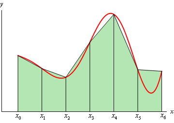 An example trapezoidal approximation of a function f(x), notated by each x interval. Courtesy of Paul's Online Notes.
$$T(x) = \frac{h_1}{2}(y_0 + y_1) + \frac{h_2}{2}(y_1 + y_2) + \dots + \frac{h_k}{2}(y_{k-1} + y_k)$$ $$h_1 = x_1 - x_0,\space\space h_2 = x_2 - x_1, \space\space\dots,\space\space h_n = x_n - x_{n-1}$$
$$T(x) = \frac{h_1}{2}(y_0 + y_1) + \frac{h_2}{2}(y_1 + y_2) + \dots + \frac{h_k}{2}(y_{k-1} + y_k)$$ $$h_1 = x_1 - x_0,\space\space h_2 = x_2 - x_1, \space\space\dots,\space\space h_n = x_n - x_{n-1}$$
#
Rule .
In the special case of the Trapezoid Rule where h is a constant: The Trapezoid Rule can be simplified to
$$T = \frac{h}{2}(y_0 + 2y_1 + 2y_2 + \dots + 2y_{n-1} + y_n)$$
where [a,b] is partitioned into n subintervals of equal length h = (b-a)/n.
# Differential Equation: A Differential Equation is an equation involving a derivative. Three types of equations are used when two variables are changing at the same time.
# Functions with Discontinuities: The general solutions found using this method are only valid for continuous functions. So if a function contains discontinuities you need to restrict the domain to the continuous portion of the function that contains the solution. In order to make a discontinuous function have a particular solution, you must restrict the domain so that the point you want is included in the domain.
# Indefinite Integrals with FTC: The family of all antiderivatives of a function f(x) is the indefinite integral of f with respect to x written: $$\int f(x)dx$$ If f is a function such that F'(x) = f(x), then $$\int f(x)dx = F(x) + c$$ , where c is an arbitrary constant, called the constant of integration. Although Definite Integrals and Indefinite Integrals look similar, they are not all alike. A definite integral is a number, the limit of a sequence of Riemann sums; also represented by the area between a curve and the x-axis. An Indefinite Integral is a family of functions havin a common derivative.
#
Rule .
DEFINITE INTEGRALS HAVE UPPER AND LOWER LIMITS AND REPRESENT THE AREA UNDER THE CURVE. Indefinite integrals just have the integrand with no limits, and they find the family of functions with a common derivative. That's why indefinite integrals have +c and definite integrals don't.
# PROPERTIES OF INDEFINITE INTEGRALS:
$$\int k \cdot f(x) dx = k \int f(x) dx$$ , where k is some constant.
$$\int (f(x) \pm g(x)) dx = \int f(x) dx \pm \int g(x) dx$$
POWER FORMULAS:
$$\int u^n du = \frac{u^{n+1}}{n+1} + c$$ , where n ≠ -1.
$$\int u^-1 du = \int \frac{1}{u} du = \ln|u| + c$$
TRIG. FORMULAS: $$\int \cos(u) du = \sin(u) + c$$ $$\int \sin(u) du = -\cos(u) + c$$ $$\int \sec^2(u) du = \tan(u) + c$$ $$\int \csc^2(u) du = -\cot(u) + c$$ $$\int \sec(u)\tan(u) du = \sec(u) + c$$ $$\int \csc(u)\cot(u) du = -\csc(u) + c$$
EXPONENTIAL FORMULAS: $$\int e^u \, du = e^u + c$$ $$\int a^u du = \frac{a}{\ln(a)} + c$$
LOGARITHMIC FORMULAS: $$\int \ln(u) = u\ln(u) - u +c$$ $$\int \log_a(u)\,du = \frac{1}{\ln(a)} \int \ln(u)\,du = \frac{u\ln|u|-u}{\ln(a)} + C$$
#
Rule .
When a problem requires you to 'verify' an antiderivative, what you want to do is start from the side that doesn't have an integral (the antiderivative), and take the derivative of it. That's all.
?. U-Substitution.
#
Rule .
Whenever you have an indefinite integral with a variable of integration different from the variable in the expression, you just have to plug in whatever value u or x is equal to into the expression to make it agree with the variable of integration. For example, where u = x²:
$$\int (u^3 + 1)dx = \int (x^6 + 1) dx$$
$$\int (u^3 + 1)dx = \int (x^6 + 1) dx$$
#
Rule .
Sometimes you don't want to plug in the value for u and you actually want to replace the variable of integration (the dx or du). The move here is to take the value of u, u=2x for example, and take the derivative of both sides: du/dx = 2. Then, multiply by dx or du, where du = 2dx, and then isolate dx. dx = du/2. Finally, plug that in for the dx in the thing.
#
Rule .
For the substitution -u business, you'll generally want u to be the exponent or wahtever makes the equation 'weird' (as in, the aspect that complicates the equation the most to not fit into one of the basic "PROPERTIES OF INDEFINITE INTEGRALS" molds). From there, take the derivative and do everything necessary to isolate dx so that the front expression can all be one variable. Then, take the antidervative as normal (since it should now have been converted into the basic molds showcased in the properties), and when you have completed it, substitute back in the value you set for u.
#
Rule .
As a final addendum to u-sub's, take into consideration how they are meant to remove as much as possible from the expression in the name of u, so how du and dx are isolated can be messed around with to be whatever. If you see anything outside of the u (which is just anything that looks chain-ruled), you can warp the middle du/dx equation to reflect what you went to take out: ⅙du = x²dx.
#
Rule .
When the x-variable in the integral are to the same degree, you must solve for x. When creating u, instead of taking the derivative right away, isolate x. For example, in a definite integral like
$$\int x \sqrt{3x+2} dx$$
, where u = 3x+2, you can establish that u-2=3x.
From there, (u-2) / 3 = x. You now have what u is equal to, so you can carry on with the rest of the substitution as normal: (du / 3) = dx. By distributing u in the expression, you will create multiple expressions in the solutions.
From there, (u-2) / 3 = x. You now have what u is equal to, so you can carry on with the rest of the substitution as normal: (du / 3) = dx. By distributing u in the expression, you will create multiple expressions in the solutions.
?. Separable Equations & Applications.
The solution is found by antiderivating both sides.
# How To Solve All Separable Equations:
Step 1: Get all "y" terms on one side.
Step 2: Get the "dx" on both sides.
Step 3: Integrate both sides in respect to each variable.
Step 4: Solve for "c" if possible.
# Exponential Change: Exponential Change occurs when the rate of change is proportional to the amount present. This is when you can multiply the amount by a factor each time to get a new amount:
y = k * x
(dy/dt) = k * y
# Compound Interest:
$$A(t) = A_0 (1+\frac{r}{k})^{kt}$$ A0 = amount invested (initial condition).
r = interest rate (decimal rate).
k = # of times per year compounded.
t = time in years (or whichever time is specified by the question)
# Modeling Growth with Other Bases: $$y = y_0 b^{\frac{-t}{n}}$$ y0b = the desired growth.
n = the amount of time until the value is multiplied by b, i.e. the length of one growth cycle.
t = time in years (or whichever time is specified by the question)
#
Rule .
For the most distilled understanding of separable equations possible, A is just going to represent moving x and y to either side any way you can. If there is no x or y, pretend it exists. For EXPONENTIAL CHANGE, the equation is:
$$y = y_0 e^{rt}$$
, where y is the total after time t, r is the rate, and y0 is the initial amount. To determine any equation, you just need to know y (generally always either y0 doubled or in 30 years), and two of either r, t, or y0. The irregular compound is the (1 + r/k) one described in the "Compound Interest" Blue Section, where r is always a decimal.
The half-life form is $$y = y_0 e^{-kt}$$ , with the half-life itself being ½y0.
The half-life form is $$y = y_0 e^{-kt}$$ , with the half-life itself being ½y0.
# Trigonometric Antiderivatives:
$$\int \sec(x) dx = \ln(|\sec(x) + \tan(x)) + c$$ $$\int \csc(x) dx = \ln(|\csc(x) - \cot(x)|) + c$$ $$\int \tan(x) dx = \ln(|\sec(x)|) + c$$ $$\int \cot(x) dx = \ln(|\sin(x)|) + c$$ $$\int \tan^2(x) dx = -x + \tan(x) + c$$ $$\int \cot^2(x) dx = -x-\cot(x)+c$$
#
Rule .
Integrating velocity gives displacement. Displacement is the net area between the velocity curve and the time x-axis.
Integrating the absolute value of velocity gives total distance traveled. Total distance is the total area between the velocity curve and the time x-axis.
When you want to find the position of a particle, you can integrate the v(t) using t as the upper limit and with the initial position, you just add the ∆s displacement (the definite integral of the integral of f(x) from 0 (or whatever) to t, added to the initial position): s(0) + ∆s. Given an integral, equation, and initial position, you just follow s(0) + ∆s, where ∆s is the integral, and you find the Displacement.
#
Rule .
In finding the total distance, remember you are finding the total ground covered. Total Distance is
$$\int_a^b |v(t)| dt$$
If necessary to do by hand, find where y=0 and use that as the splitter for two definite integrals. Then solve.
#
Rule .
Area Between Curves:
If f and are continuous functions with f(x) ≥ g(x) on [a,b], then the area between the curves y = f(x) and y = g(x) from a to b is the integral of [f-g] from a to b:
$$\int_a^b (f(x) - g(x)) dx$$
$$\int_a^b \text{“top - bottom”}\,dx$$
For example, if a question asked you to determine the area of the region between y = sec²(x) and y = sin(x) on [0, π/4], you would solve as follows:
Step 1: Graph the curves to find their relative positions in the plane.
The positions of y = sec²(x) and y = sin(x) between 0 and π/4. Courtesy of Paul's Online Notes.
Step 2: Write an integral and solve. $$A = \int_a^b f(x) - g(x) dx$$ $$A = \int_0^{\frac{\pi}{4}} \sec^2(x)-\sin(x)dx$$ Reminder that f(x) will always be the one above the g(x).
For example, if a question asked you to determine the area of the region between y = sec²(x) and y = sin(x) on [0, π/4], you would solve as follows:
Step 1: Graph the curves to find their relative positions in the plane.
Step 2: Write an integral and solve. $$A = \int_a^b f(x) - g(x) dx$$ $$A = \int_0^{\frac{\pi}{4}} \sec^2(x)-\sin(x)dx$$ Reminder that f(x) will always be the one above the g(x).
#
Rule .
Areas enclosed by intersecting curves: When a region is enclosed by intersecting curves, the points of intersection give the limits of integration. You can find the individual zeroes by setting the functiosn equal to zero, but setting the functions equal to eachother will proivde the intersection points.
For example: Determine the area of the region enclosed by the Parabola y = 2-x² and the line y = -x.
Step 1: Graph the curves (determine f(x) & g(x)).
Step 2: Determine the intersection either algebraically or using a calculator. Set the functions equal to eachother and solve:
2-x² = -x
0 = x² - x + 2
0 = (x - 2)(x + 1)
x = 2, x = -1
These values represent the limits of the integral.
Step 3: Set up using integral & solve: $$\int_{-1}^2 (2-x^2-(-x)) dx$$ $$= \int_{-1}^2 (2+x-x^2) dx$$ $$\left[2x + \frac{x^2}{2} - \frac{x^3}{3}\right]_{-1}^{2}$$ $$= 4 + 2 - \frac{8}{3} - (-2 + \frac{1}{2} - \frac{-1}{3})$$ $$= \frac{18}{3} - \frac{8}{3} - (\frac{-7}{6})$$ $$= \frac{20}{6} + \frac{7}{6}$$ $$\boxed{ \int_{-1}^{2} (2+x-x^2)\,dx = \frac{27}{6} \space \text{units}^2}$$
#
Rule .
For those issues where part of the graph isn't touching the second function and part is (i.e., separate bounds for different parts of the full area, like the shape given by y=0, y=√x, & y=x-2), just set the second function equal to zero to find the zeroes and integrate each side separately.
#
Rule .
When you have to choose to integrate with respect to x or y, choose whichever one is easier and doesn't require a ±.
#
Rule .
VOLUME OF A SOLID:
The volume of a solid of a known integrable cross-section of area A(x) from x=a to x=b is the integral of A from a to b. Here is the method to find it:
Method:
For an example of a square cross-section: A pyramid 3 m high has congruent trinagular sides and a square base that is 3m on each side. Each cross-section of the pyramid parallel to the base is a square. Determine the volume of the pyramid.
The volume of a solid of a known integrable cross-section of area A(x) from x=a to x=b is the integral of A from a to b. Here is the method to find it:
Method:
- Sketch the solid and cross-section A(x).
- Determine a formula for f(x) = area of cross-section.
- Determine limits of integration (a and b).
- Integrate A(x) to determine volume.
For an example of a square cross-section: A pyramid 3 m high has congruent trinagular sides and a square base that is 3m on each side. Each cross-section of the pyramid parallel to the base is a square. Determine the volume of the pyramid.
- Sketch/Visualize:
TA semi-3-dimensional graph of the described pyramid under the given bounds, with the vertex at the origin and an example cross-section. Courtesy of West Shore School District.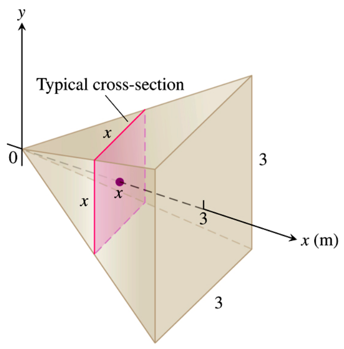
- A(x) = area of cross-section, where each cross-section is a square. Thus, the equation for A(x) = (x)(x) = x²
- Limits of Integration: We are taking cross-sections as we move up the height of the pyramid, so the limits are 0 ≤ x ≤ 3.
- Integrate: $$\int_0^3 x^2 dx$$ $$= \left[ \frac{x^3}{3} \right]_{0}^{3}$$ $$\boxed{ = \frac{27}{9} = 9}$$
#
Rule .
For many volume-integration problems, the variables will be coded into the question: "The solid lies between planes perpendicular to the x-axis at x=-1 and x=1". The two numbers given here will be your limits of integration.
"...run from y=-√x to y=√x". These are the functions that will serve as the bounds for the cross-section.
There are several caveats here: if the text before says the shape, use that in the mathematics.
"...run from y=-√x to y=√x". These are the functions that will serve as the bounds for the cross-section.
There are several caveats here: if the text before says the shape, use that in the mathematics.