
This is the first part of my complete notes for Electromagnetism, covering topics of Electrostatics such as Electric Charge, the Law of Electric Force, Conduction/Induction, Electric Fields, Electric Flux, Gauss's Law, and more.
I color-coded my notes according to their meaning - for a complete reference for each type of note, see here (also available in the sidebar). All of the knowledge present in these notes has been filtered through my personal explanations for them, the result of my attempts to understand and study them from my classes and online courses. In the unlikely event there are any egregious errors, contact me at jdlacabe@berkeley.edu.
Summary of Electromagnetism, Part 1: Electrostatics
Table Of Contents
XII. Law of Electric Force.
XII.I Electric Charge.
The character 'q' is used to denote the net charge on an object.
#
P. Rule .
The 'Coulomb' is the SI unit for Electric Charge. Specifically, it is defined as the "amount of electric charge transported by a current of one ampere flowing for one second" (see definitions of each new term, they are gone over in more depth later on).
By itself, a Coulomb is a huge amount of charge - charged particles like protons and electrons have electric charges many orders of magnitude smaller than a single Coulomb. Two objects, each with one Coulomb of charge, located one meter apart, experience an electric force (see Subsection XII.III) of roughly nine billion Newtons.
By itself, a Coulomb is a huge amount of charge - charged particles like protons and electrons have electric charges many orders of magnitude smaller than a single Coulomb. Two objects, each with one Coulomb of charge, located one meter apart, experience an electric force (see Subsection XII.III) of roughly nine billion Newtons.
# Excess Charge: The state of an object being more positively or negatively charged due to a lack or oversupply of negatively-charged electrons, the movement of which can be facilitated by rubbing objects together (charging by friction). Since positive ions are fixed in place, an object can only change in charge through the removal or addition of negative charges.
An "excess positive charge" is slang for an electron deficit, while an "excess negative charge" means an oversupply of electrons.
Note that the excess charge is effectively the total charge of the object, considering how an object without excess charge is considered to have a net-zero charge (neutral).
# Law of Charges:
Opposite charges attract, while like charges repel.
Example: Rubbing a balloon against one's hair will cause the electrons to move from the hair to the balloon (a transfer faciliated by rubbing), causing the balloon to stick to the hair. Furthermore, since each hair will become more positively-charged, they will repel one another, causing one's hair to stick up and separate.
XII.II Basics of Atomic Physics.
#
P. Rule .
An atom is the smallest unit of matter retaining the chemical properties of its element. It is composed of a dense nucleus with Protons and Neutrons, and surrounded by orbitals of Electrons.
Electrons & Protons are small particles (e.g., specks of mass) that carry an electric charge with a magnitude of ~1.602 × 10⁻¹⁹ Coulombs, which is referred to as the "Elementary Charge". Protons are positively charged, while electrons are negatively charged.
Electrons are elementary particles, indivisible by nature, while protons and neutrons are composed of quarks, the REAL smallest particles. Specifically, the proton has two up quarks and one down quark.
The up quark has a charge of +(2/3)e, while the down quark has the charge -(1/3)e. Thus, the net quark of a proton is +e.
The neutron, being composed of one up quark and two down quarks, has a net charge of 0. If this were not the case, the neutron would not be electrically neutral, and the nucleus of an atom would tear apart as the protons would repel from one another without the stabilizing force of the neutrons.
The electron, being an elementary particle (defined below), just has a net charge of -e.
# Elementary Charge: An electrical charge of 1.602 × 10⁻¹⁹ Coulombs, the standard charge of Protons and Electrons and the smallest charge recorded on an isolated particle (quarks aren't isolated). Represented as 'e'.
# MElectron (Electron Mass): 9.11 × 10⁻³¹ kg.
# MProton (Proton Mass): 1.67 × 10⁻²⁷ kg. This is over 1800x greater than the mass of an electron.
#
P. Rule .
There is an equation relating net charge and elementary charge (or any quantifiable proportion of elementary charge), useful for determining how many excess charge carriers it would take for a specific net charge to be achieved:
q = n × e
q = Net charge on an object.
n = Excess number of charge carriers (protons or electrons or whatever - it just has to be ONE of them).
e = The Elementary Charge Constant.
q = n × e
q = Net charge on an object.
n = Excess number of charge carriers (protons or electrons or whatever - it just has to be ONE of them).
e = The Elementary Charge Constant.
#
P. Rule .
Charge is quantized, meaning that it must come in discrete quantities, integer multiples of the elementary charge. This is because the 'net charge' of an object is the product of having more or fewer charged particles, and thus only multiples of the elementary charge are possible (since elementary particles are indivisible).
Using the net/elementary charge relation (see Rule 160), one can find that it is impossible for an object to have a net negative charge of 2.00 × 10⁻¹⁹ Coulombs, as such a net force would require 1.25 electrons, violating quantization.
Using the net/elementary charge relation (see Rule 160), one can find that it is impossible for an object to have a net negative charge of 2.00 × 10⁻¹⁹ Coulombs, as such a net force would require 1.25 electrons, violating quantization.
#
P. Rule .
When the atoms of a conductor form a solid, some of their outermost (and most loosely held) electrons become free to wander about within the solid, leaving behind positively charged atoms (positive ions). These wandering electrons are known as conduction electrons. There are practically no free electrons in a nonconductor, since those electrons are tightly bound to their atoms.
Knowledge of the "mobility of charge" within conductors, and conductors alone, is fundamental for comprehending concepts in Electric Field and Charge-Flux Law type questions - see Rule 170.
Knowledge of the "mobility of charge" within conductors, and conductors alone, is fundamental for comprehending concepts in Electric Field and Charge-Flux Law type questions - see Rule 170.
XII.III Electric Force.
# Electroscope: An instrument for demonstrating electric charge. They take several forms, but generally have some place where an isolated charge (protected by some insulator, like glass) is held.
#
P. Rule .
Law of Electric Force (Coulomb's Law) (8): VECTOR.
Units: Newtons.
Equation:
Fe = (k × q1 × q2) / (r²)
Fe = The magnitude of the electric force that exists between two charged particles.
k = The Coulomb constant, equal to 8.99 × 10⁹ (N × m²) / (C²).
q1 = The net charge on object 1, measured in Coulombs.
q2 = The net charge on object 2, measured in Coulombs.
r = The distance between the centers of charge of the two objects.
Definition: Coulomb's Law, hereafter referred to as the Law of Electric Force, enables one to find the magnitude of the Electric Force with respect to two particles.
Note that this equation looks very similar to the Universal Law of Gravitation (see Rule 140). Accordingly, k (the Coulomb constant) functions similar to G (the Gravitational constant), being equal to (N × m²) / (a particular composition property of mass)². Clearly, since the Coulomb constant is 20 orders of magnitude stronger than the Gravitational constant, the Electric Force between objects is much more powerful than their Gravitational attraction. Fe >>> Fg.
If the calculated Electric Force has a Negative Value, then it is an attractive force. If the Electric Force has a Positive Value, then it is a repulsive force. This is quite obvious upon momentary consideration - a negative and a positive charge will always produce a negative, and thus attractive force, which matches the Law of Charges that opposite's attract. Thus also follows for repulsive like charges.
# Attractive Force: A force that pulls entities together, whether masses or charges.
# Repulsive Force: A force that pushes entities apart.
# Point Charge: An object with zero size (an infinitely small dot) that carries an electric charge. This can be generalized to any object whose mass is negligible compared to its charge. It is the Electric equivalent to a 'point mass', in that a particular charge is concentrated upon a single particle/point in space for the purpose demonstrating physical properties.
# MicroCoulombs (μC): One one millionth of a Coulomb. E.g., 1 × 10⁻⁶ C. Occasionally misstated as "Myu Coulombs", "Myu-Coulombs", etc.
# NanoCoulombs (nC): One one billionth of a Coulomb. E.g., 1 × 10⁻⁹ C.
# PicoCoulombs (pC): One one trillionth of a Coulomb. E.g., 1 × 10⁻¹² C.
#
P. Rule .
With charges, the fundamental concept to understand in applying the Law of Electric Force is that in order to derive any useful information (depending on the question, but in general), you must determine the effect of the electric force on the individual point charges. Specifically, you must be able to determine the direction the charges will move in as a result of the force.
The Law of Electric Force determines the repulsive or attractive force acting on both charges, since they are a Newton's Law Force Pair (see Rule 74). However, in addition, you must utilize this information to determine the direction of the movement of each charge. If you have a proton on the left and an electron on the right, the proton will move rightward and the electron leftward as they attract toward one another. If you have two electrons, they will move in opposite directions away from one another.
The Law of Electric Force determines the repulsive or attractive force acting on both charges, since they are a Newton's Law Force Pair (see Rule 74). However, in addition, you must utilize this information to determine the direction of the movement of each charge. If you have a proton on the left and an electron on the right, the proton will move rightward and the electron leftward as they attract toward one another. If you have two electrons, they will move in opposite directions away from one another.
# Permittivity of Free Space:
There is a concept known as Electric Permittivity that is discussed in Section XVI, Rule 212. It is an attribute that fluctuates in value from problem to problem according to its equation. It essentially measures the Polarization (Rule 169) of a specific type of material (a dielectric, see Rule 216), and will be discussed more fully at a later time.
What can be revealed right now, and what will become fundamental for future sections, is the "Permittivity of Free Space", a constant value that measures how dense an electric field (in relation to an electric charge) will be "permitted" to form within a vacuum. Thus, all equations that use the constant imply that the electric field is being formed within a vacuum.
The Permittivity of Free Space is referred to as "Epsilon Naught" verbally, and has the following value:
ε0 = 8.85 × 10⁻¹² (C²) / (N × m²).
This little constant will be used everywhere. It will become ubiquitous in electromagnetism. You will forget you ever lived without it, that there ever existed a time that it was not a fundamental part of your existence, and you will feel closer to it with each passing problem.
#
P. Rule .
Coulomb's constant: SCALAR (a constant).
Units: (C²) / (N × m²), using Columbs, Newtons, and Meters.
Equation:
k = (1 / 4πε0)
k = The Coulomb constant, equal to 8.99 × 10⁹ (N × m²) / (C²).
ε0 = "Epsilon Naught", The Permittivity of Free Space, equal to 8.85 × 10⁻¹² (C²) / (N × m²).
Definition: The Coulomb Constant, 'k', 8.99 × 10⁹ (N × m²) / (C²), used in such equations as the Law of Electric Force (see Rule 163) and all its applications, has a special fixed relationship with another constant. This other constant is the permittivity constant, also just known as the permittivity of free space (described above).
This equation, of course, can be substituted in for 'k' wherever applicable. Furthermore, ε0 itself, as described in the "Permittivity of Free Space" blue section above, appears in several equations by itself, most notably the Charge-Flux Law (see Rule 188). The reasons for the usage of Coulomb's Constant at all is a matter of antiquated historical decisioning that we have to live with today.
# Isolated System: A system is isolated when charges are not able to enter nor exit the system. The universe, being isolated, has a constant net charge.
#
P. Rule .
Conservation of Charge:
The total electric charge of an isolated system never changes.
qi total = qf total
If the conductors being touched in a conservation of charge-type equation are identical (in all manners other than charge), then the excess charge will be evenly distributed between the two conductors. For example, if there are two conductors, one with a charge of -3 nC and the other with +6 nC, then the final charge of each conductor, once touched, will be 1.5 nC.
# Electricity: The flow of electrons through a conductor.
# Conductor: Something that can conduct electricity, like a wire. On the outside of a wire, there is rubber or plastic that serves as an insulator/nonconductor: something that doesn't conduct electricity very well or at all.
# Semiconductor: A material that holds both qualities of a conductor and insulator and can be tailored to be a better conductor or insulator. Depending on electrical signals, it can be conducting or insulating. Examples: Silicon, Germanium.
# Superconductor: An idealized perfect conductor, allowing charge to move without any hindrance.
#
P. Rule .
GROUND.
All excess charges can quickly be diffused through the usage of a Ground. A Ground is any sort of release point (if excess negative) or gain point (if excess positive) for the excess charges of a system: an ideal ground is an infinite well (see VII.VI) of charge carriers - such a requirement is effectively met by the Earth.
An Earth Ground is created when a circuit has a physical connection to the earth, in order to sink (lose) or source (obtain) electrons through the earth itself. The Earth has a practically infinite number of electrons that can be used to balance out a circuit/system, pulling from or giving to it. Relative to very small charged systems, the human skin could serve as a ground as well.
The end result of a ground is an electrically neutral system.
In electrical engineering, all circuits require a Ground to function - it is often referred to as "GND", and has its own symbol for use in diagrams (see E.E. Rule [[[). In many electrical situations, without the availability of a physical connection to the Earth, a "Floating Ground" can be used, which simply serves as a type of '0V reference line' (see def. of Voltage) that acts as a return path for current back to the negative side of the power supply.
#
P. Rule .
There are two distinct categories, processes under which charge is transferred. Specific means of transfer, like charging by friction (rubbing) fall under these wider processes. These processes are Conduction, and Induction.
Conduction:
This is the transfer of charge in which current flows because of the electric field. There are only two requisites for an object to be charged by conduction, through another object:
1. The objects have to touch.
2. The objects must, after touching, have the same sign of net charge.
Induction:
This is the transfer of charge in which a changing magnetic field generates an electromotive force (see Rule [[[), resulting in an induced charge. It is not important to fully understand what an "electromotive force" is right now, just that it is the electric force that drives current through a circuit.
There are only two requisites for an object to be charged by conduction, and they are the eact opposite of conduction:
1. The objects do not touch.
2. The objects must finish with opposite signs of net charge.
#
P. Rule .
Polarization:
Polarization is the process through which the charges within objects (and thus their associated particles) align themselves in such a way that there becomes a net attractive force, as a result of attraction & repulsion from an object with excess charge.
Polarization doesn't change the net charge of the object, but rather has to do with how charges rearrange themselves within the object.
The process itself is simple: When an object with an excess charge approaches a neutral object, the like charges will repel and the opposite charges will attract (the electrons being the sole moving particles, moving either in front of or behind the protons). Since the opposite charges will be closer to the charges of the object than the like charges, by the Law of Electric Force, there will be a net attractive electric force, since the opposite charges have a smaller 'r' value than the like charges.
This is the reason that balloons stick to walls once they have an excess negative charge. The wall, as an insulator without free electrons, cannot "attract" the charge of the balloon. Instead, the charges in the wall rearrange themselves and end up with that net attractive force.
Electric force due to polarization is small - objects with small masses, like balloons and aluminum cans, can be held in place and rolled respectively using only a small electric force.
Electric force caused by the polarization of a conductor is typically larger than a polarized insulator. This is because electrons in insulators are bound in their atoms, while electrons in conductors are able to move to the opposite side of the object.
For information as to how polarization can be used to the advantage of a capacitor (Section XVI), see Rule 216.
#
P. Rule .
Placement of Charge within Conductors & Nonconductors:
The nature & positioning of the charge within the thickness of an object (like a shell or thick cylinder) differs depending on whether the material of the object is a conductor or insulator.
Conductive objects (enclosed shapes) spread out all excess charge (read: electrons) over their external surface. This is because the conduction electrons of the conductor (see Rule 162) and the excess charge electrons will repel from one another, causing the excess charge electrons to spread over and distribute across the farthest possible surface.
If the object is symmetrically shaped, like a sphere, this distribution will be uniform. Otherwise, if the object is irregularly shaped, then surface charge density will vary and have specific maximums - see Rule 196 for a complete description.
!!!NOTE!!!: Unless the conductor is circular (spherical or cylindrical), the charge will not distribute itself uniformly. This is a matter of symmetricality, an attribute that leads circular objects (shell or solid) to naturally become uniformly distributed in charge, but not any other shape. This is not to say that a question will not simply say "assume a uniform charge density" for some ridiculous, noncircular shape, violating the laws of physics for the sake of examining the physicist. In such a case, you would do as told and use the given information appropriately. The surface charge density σ (charge per unit area) varies over the surface of any noncircular conductor. The electric field (see Section XIII) immediately outside of the surface of the noncircular shape can be determined quite easily however, as described in Rule 197.
This concentration of charge on the external surface is the same for both positive and negative excess charge. If there is an excess positive charge (imagine the conduction electrons have been removed), then the positive charge will then spread uniformly across the surface. In other words, the "absence of electrons" will be uniformly distributed.
In the state of uniform charge distribution, the conductor will be in a state of electrostatic equilibrium - see Rule 194 for a complete explanation involving Electric Fields.
Nonconductive/Insulating objects (enclosed shapes), which do not allow free movement of charge, bind electrons to their atoms and thus do not move to redistribute excess charge. When an excess charge is added, there are conduction electrons that would even allow for the charge to be moved, and so the excess charge will simply remain wherever it is placed.
Thus, the excess charge can be uniformly distributed if that is the state in which it is added, and questions oftentime instruct the physicist to assume such a condition. However, if the charge is concentrated in a particular region, it will not naturally redistribute itself as it would in a conductor.
For a continuation of this Rule, with respect to how the conductor/nonconductor dispersal of charge affects electric field distribution, see Rule 194.
#
P. Rule .
Shell Theorems of Electric Force:
Shells, spherical or cylindrical entities of a specified thickness and a hollow interior (like a ring rotated 180° along the x-axis, with the thickness being ≥0), retain the same importance they had in Mechanics for Electromagnetism.
Akin to the Shell Theorem for Internal Gravitation (see Rule 149), there are TWO Shell Theorems for Electric Fields - yet another similarity between electric force and gravitational force (see Rule 163 for the first). They are relatively straightforward, but are only applicable under the specified conditions.
These theorems literally do not work for any shape other than a shell/sphere - there is a particular symmetry with those specific shapes that allow these theorems to be used. They are not true for just any irregular, wack shape.
Fundamental to the understanding of these theorems is the nature of charge distribution on shells, which itself depends on whether the shell is conductive or not. See Rule 170 for a full, generalized treatment of these principles. Nonconductive shells are not in a state of electrostatic equilibrium (see Rule 194), unlike Conductive shells.
- A charged particle outside of a shell with charge uniformly distributed on its surface (e.g., a conductor) is attracted or repelled as if the shell’s charge were concentrated as a particle at its center. This is assuming the charge on the shell is much greater than the charge of the particle, thus not interfering with the distribution of charge on the shell (an issue detailed in Rule 170).
- A charged particle inside a shell with charge uniformly distributed on its surface (e.g., any conductor, and any nonconstructor created in such a way) will have no net force acting on it due to the shell.
XIII. Electric Fields.
XIII.I Introduction to Fields.
If the test charge is positive, then it will be in the same direction as the electric field, and if it is negative, then it will be in the opposite direction of the electric field. By convention, positive test charges are used to define electric fields.
#
P. Rule .
Electric Field: VECTOR.
Units: Newtons / Coulombs.
Equation:
E = (Fe / q)
E = The magnitude of the electric field at a particular point.
Fe = The electric force being felt by the charge at the particular point being measured.
q = The magnitude of the charge/charged particle of the particular point being measured.
Definition: An Electric Field is a field in space surrounding a charged object, in which the object's electric force has strength.
Electric fields have their direction expressed in the form of lines, the nature of which is elucidated in Rule 174. Naturally (meaning without the interference of another electric field), these lines, which originate at every point of the object's surface, will be perpendicular to the object and will point radially outward or inward (depending on the charge sign) forever without bending - the electric field of a point charge, for example, will shoot off in every direction in such a way. The direction and lines themselves, however, can be influenced as a result of the Law of Charges and can bend accordingly - see Rule 174.
Technically, the given equation dictates that the electric field is the "amount of electric force per charge at a point in space", the ratio between the electric force of the charge and the magnitude of the charge itself. All charge creates an electric field in relation to its electric force.
The reason an exact magnitude value can be determined for an electric field (an inherently emanating and changing entity), as is done in the given equation, is because the magnitude being found is that of the strength of electric field at a particular point, denoted by the electric force experienced by the charge placed at that point.
# Uniform Electric Field: An electric field that has the same magnitude and direction at every point within the field - think of the electric field created by an infinitely long pole. These electric fields, of course, are overtly idealized.
#
P. Rule .
The magnitude of the electric field will decrease as the test charge gets farther from the point charge, as a result of the Law of Electric Force (since the denominator distance value increases and all). The electric field surrounding (and caused by) a point charge is constant at a constant radius from the point charge.
The entire Law of Electric Force equation can be substituted into the Electric Field equation, enabling one to simplify things considerably if the circumstances allow.
The entire Law of Electric Force equation can be substituted into the Electric Field equation, enabling one to simplify things considerably if the circumstances allow.
#
P. Rule .
Electric Field Lines:
1. The lines of attraction in an electric field always point away from the positive charge (origination) and toward the negative charge (termination). Thus, the lines always point in the direction in which the test charge would experience an electric force.
2. The # of electric field lines per unit area is proportional to the electric field strength. Therefore, a higher density of electric field lines means a higher electric field strength.
3. Electric field lines always start perpendicularly to the surface of the charge, and start on a positive charge and end on a negative charge (unless there is more of one charge, in which case some lines would start/end infinitely far away).
4. Electric field lines never cross.
Use the test charge (a positive entity - see the definition) as the sample particle, for the sake of illustrating this point.
When the test charge (standardized as positive) is placed in the field of a positive point charge, the test charge will be repelled from the point charge. Electric force projects radially outward from the positive point charge, decreasing in magnitude as distance increases.
On the flip side, if the point charge is negative, then the test charge will be attracted toward the point charge. All of the arrows will point radially inward toward the negative point charge.
XIII.II Continuous Charge Distributions.
λ = (Q / L)
λ = (Lambda) The direction and magnitude of the given expression, defined in Coulombs per Meter (C / m).
Q = The charge of the object.
L = The length of the object - this form of density is best applied to charge along a flat line.
Treat λ as a constant when taking the derivative. Note, however, that the given equation can be transmuted into a derivative form: λ = (dQ / dL). This is because the ratio remains the same: total charge divided by total length is equal to the infinitesimally small individual charge over the length thereof.
# Surface Charge Density:
σ = (Q / A)
σ = (Sigma) The direction and magnitude of the given expression, defined in Coulombs per Meter Squared (C / m²).
Q = The charge of the object.
A = The total area of the object.
Treat σ as a constant when taking the derivative. Note, however, that the given equation can be transmuted into a derivative form: σ = (dQ / dA). This is because the ratio remains the same: total charge divided by total area is equal to the infinitesimally small individual charge over the area thereof.
# Volumetric Charge Density:
ρ = (Q / V)
ρ = (Rho) The direction and magnitude of the given expression, defined in Coulombs per Meter Cubed (C / m³).
Q = The charge of the object.
V = The total volume of the object.
Treat ρ as a constant when taking the derivative. Note, however, that the given equation can be transmuted into a derivative form: ρ = (dQ / dV). This is because the ratio remains the same: total charge divided by total volume is equal to the infinitesimally small individual charge over the volume thereof.
#
P. Rule .
Electric Field of a Continuous Charge Distribution (CCD): VECTOR.
Units: Newtons / Coulombs. It is a type of electric field.
Equation:
$$E_{CCD} = k \int \frac{dq}{r^2} \hat{r}$$
ECCD = The electric field that exists around a continuous charge distribution, calculated at point r in space.
k = The Coulomb constant, equal to 8.99 × 10⁹ (N × m²) / (C²).
dq = The infinitesimally small point charges, of which there is an infinite number of. This value can be substituted for any of the equivalent charge density derivatives (see Linear, Surface, and Volumetric), pursuant to the nature of a particular problem.
r = The distance between the infinitesimal charge dq and the point where the electric field is being calculated. Unlike the Law of Electric Force, this r is a function that varies depending on the charge, since there is technically an infinite number of charges (dq).
r̂ = The unit vector pointing from dq (whichever charge) toward the test charge - this is most applicable post-integral, when you can have a test charge to calculate the strength of the electric field with respect to. The direction points radially outward for positive dq, and inward for negative dq.
Definition: A Continuous Charge Distribution (CCD) is a simple concept that elaborates the simple 'point' model of charges into one that uses calculus to account for more chargetype possibilities, furthering the infinite journey into human knowledge.
A 'continuous charge distribution' is simply a charge that isn't a point charge; e.g., a charge with a shape and an electric charge continuously distributed throughout the object.
The electric field that exists around a continuous charge distribution can be determined through a rethinking of the standard Electric Field-Law of Electric Force combined equation (see Rule 172) using Calculus. Since the charged object is made up of an infinite number of infinitesimally small point charges ('dq' representing them individually), the therefore infinite number of electric fields can be calculated using an integral.
There are very specific use cases for this integral: it is not applicable everywhere. See Rule 176 for a detailed treatise on this cases and their exceptions. The limits of integration of the integral are specific to each problem and can be determined through ingenuity and through the power of the indomitable human spirit.
That pesky 'dq' thing can be switched out by taking the derivative of any of the charge densities (see linear, surface, and volumetric), depending on what one is looking for.
The Electric Potential created by a CCD has a near identical equation to its electric field, described in Rule 206.
#
P. Rule .
The integral equation for CCDs (continuous charge distributions, see Rule 175) is only applicable when every infinitesimal charge has its electric field pointing in the same direction when it is pointing toward the test point. For example: when the CCD is a flat line, and the test charge is on its same axis.
There are some workarounds in which the above stipulation is technically still respected, allowing the integral to still be used even for shapes like rings. This is when all components in all other directions cancel out, leaving only the components in a specific direction. For example, in a uniformly charged ring, the horizontal components of the field from symmetric charge elements cancel, leaving only the vertical (axial) component.
When all fails, and the direction of the electric at test charge P is simply not the same for every charge dq on the ring, then take the derivative of both sides of the equation (giving dE) and try to see if any components cancel eachother out anywhere - in order to find the components, use the direction of the electric field from or toward the test charge (remember: the direction points radially outward for positive dq, and inward for negative dq), and imagine that beyond the test charge or dq, wherever the direction points, the direction line continues - this extended line segment represents dE, which can then be broken into components (which will hopefully cancel out in one direction). If there are equal negative and positive dq's in a particular direction, then it cancels out. Ideally, the direction that doesn't cancel out should only a single sign no matter the direction/origin of the dq.
Generally, the dq electric field values in a particular direction 'cancelling out' is the result of a symmetry created by the placement of the point charge. For example, a point charge placed somewhere along the axis of the center of the ring.
If one has succeeded in cancelling out, then they would be able to proceed with all the necessary moving of sines or cosines (resultant from the components) and the general transfiguration of terms dependent on the characteristics of the problem itself. After one has been able to simplfy and reduce everything into only one real variable on one side (every other symbol just being a constant), then both sides can be integrated, creating a problem-specific version of the hyper-generalized CCD integral equation (see Rule 175).
All this component business requires that there be some reference position, a known x-axis and y-axis positioning in relation to the given CCD and point charge that can be used to derive the components from.
#
P. Rule .
Note that the farther you get from a finite continuous charge distribution, the more the electric field caused by the CCD matches the electric field caused by a point charge (as in, the simplified Law of Electric Force + Electric Force equation from way back when (see Rule 173)). Of course, this requires the distance between the test charge and the CCD to be much much greater than the internal distance with the CCD itself.
#
P. Rule .
Always be aware of what constants/variables are much much greater than others. In end game integrals, such as in CCD-type problems (see Rule 176), this can totally simplify whole entire parts of your equation by just thinking of the lesser variable as zero (where it is left alone and not acting as a coefficient). Of course, this mandates the usage of the approximation symbol (≈) for your answer.
#
P. Rule .
You can never assume that the equation for the electric field of a shape, whether 2d or 3d, will be the same if the shape is a conductor or a nonconductor. The world is not such a simple, idealistic place, even in what is essentially toy model physics (classical electromagnetism).
The key factor in determining whether the electric field equation for a shape is the same or differing between conductors and nonconductors, is how the charge distributes within the shape.
The following characteristics are indicative of identical equations between the electric field equations of a conductor and nonconductor shape:
The following characteristics are indicative of differing equations between the electric field equations of a conductor and nonconductor shape:
The key factor in determining whether the electric field equation for a shape is the same or differing between conductors and nonconductors, is how the charge distributes within the shape.
The following characteristics are indicative of identical equations between the electric field equations of a conductor and nonconductor shape:
- Infinite Reach: If the shape is infinite (like infinite planes or cylinders), then both conductors and nonconductors produce the same electric field at points sufficiently far from the charge distribution. Example: Infinite planes as explained in Rule 180.
- Symmetric Charge Distributions: There are cases in which some form of symmetry causes the charge distribution to remain unchanged between the conductor and nonconductor.
For example: an infinite line of charge with uniform charge density λ produced the same radial field for both conductors and nonconductors, since, being a line, the charge is "on the surface" regardless of the conductivity of the shape (in terms of how the charge being on the surface is an important distinction between conductors and nonconductors and alters the calculation of their electric fields - see Rule 170), and is emanating outward in the same fashion. - External Field Only: If only the electric field outside of an enclosed shape is being considered, then IF SYMMETRY DICTATES A FIXED CHARGE DISTRIBUTION (like shells and spheres and cylinders and whatnot, not just any wack enclosed shape), then the equation for that electrical field in particular will be the same whether the shape material is a conductor or nonconductor. This is more due to the first shell theorem (see Rule 171) than anything.
The following characteristics are indicative of differing equations between the electric field equations of a conductor and nonconductor shape:
- Internal Charge within Enclosed Shapes: As everyone knows, the charge within an enclosed shape for conductors and nonconductors differs as a result of charge placement in the solid part of the shape (like the shell part of a hollow shell) - see Rule 170. Conductors have zero electric field within themselves, and nonconductors do have some.
- Non-Uniform Charge Distribution: Conductors force charge to redistribute, whereas insulators allow charge to remain fixed. For example: a finite conducting "slab" (like a brick) with excess charge will concentrate charge at the edges, while a nonconductor could have uniform volume charge density.
This will cause differing internal and external electric fields, both for the reason outlined in Difference Characteristic #1 (directly above) and for not meeting the symmetricality requirement of Equivalence Characteristic #3 (further above).
#
P. Rule .
Flat Disks & Infinite Planes: VECTORS.
Units: Newtons / Coulombs. They are types of electric fields.
Equation:
$$E_{disk} = \frac{\sigma}{2\varepsilon_0} \left( 1 - \frac{z}{\sqrt{z^2 + R^2}} \right)$$ $$E_{plane} = \frac{\sigma}{2\varepsilon_0}$$
Edisk = The magnitude of the electric field produced by a uniformly charged flat disk, calculated at some point z from the central axis of said disk.
Eplane = The magnitude of the electric field of an infinite plane, independent of distance from the plane (interestingly).
σ = Surface charge density. See treatise here.
ε0 = The Permittivity of Free Space, equal to 8.85 × 10⁻¹² (C²) / (N × m²).
z = The distance (along the central axis) between the point at which the electric field is being measured, and the center of the disk. z ≥ 0.
R = The radius of the disk.
Definition: The Electric Field due to a (flat) uniformly charged disk and due to an infinite sheet are, in fact, closely related, the latter effectively being derived from the former.
The first equation gives the electric field magnitude on the central axis through a flat, circular, uniformly charged disk. The equation is derived in a highly logical and annoying manner, found here (offsite).
If one were to plug in infinity for R, letting the radius rise to infinity while keeping the z value finite, then the equation would simplify to that of the equation for the electric field of an infinite plane, the second given equation. By their very nature, all fields produced by infinite planes will be uniform, and thus will not change with respect to distance. The straight, parallel field lines will neither converge nor diverge from their source (the plane), and as such the field intensity will never change. READ: Electric Field is Uniform when created by a plane.
Note that despite the equation specifically being for disks and circular 2d shapes, the very act of making the radius infinite will create a plane, and thus makes its circular origins irrelevant.
By virtue of the shape being infinite (passing Equivalence Characteristic #1, see Rule 179), the infinite plane equation is true for both conductor and nonconductor infinite planes. Furthermore, know that it is also the equation for the electric field at the surface of a nonconductor, as explained in Rule 197.
XIII.III Dipole Moment.
#
P. Rule .
Electric Dipole, Electric Field (along dipole axis): VECTOR.
Units: Newtons / Coulombs. It is a type of electric field.
Equation:
Edipole = (1 / 2πε0) × (qd / z³)
Edipole = The electric field produced by a dipole along its axis, calculated with respect to the distance between the test charge and the dipole midpoint.
ε0 = The Permittivity of Free Space, equal to 8.85 × 10⁻¹² (C²) / (N × m²).
q = The absolute value of the charge of either particle.
d = The distance between the particles.
z = The distance between the test charge (the point at which the electric field is being calculated, which, being somewhere on the dipole axis, will be directly above or below the particles) and the dipole midpoint (d/2). z MUST be >>> to d, for reasons detailed in the proof (see below).
Definition: An Electric Dipole is an arrangement of two particles (point charges) with equal charge magnitudes but opposite signs. The particles are separated by distance d and lie along the dipole axis, an axis of symmetry going through both particles.
A simple graphic of what this entails is seen below:
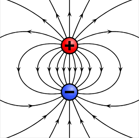 An example dipole moment, with the dipole axis running straight through the center.
The equation for the electric field produced by a dipole along its axis (and NOWHERE ELSE) is presented above. The electric field created at other points involves much more difficult, graduate-level math (offsite), and thus is dealt with much later in Physics (see Rule [[[).
There is a simple proof of the given equation, done through finding the strength of the net electric field produced by the two particles at an arbitrary point P (the test charge) along the dipole axis. It can be found here (onsite).
The internal force on the electric dipole (Fnet) will equal to zero, since the attractive forces between the particles are equal and opposite in magnitude, forming a Newton's Third Law Force Pair. They will thus be in equilibrium.
The product qd on the right side of the equation is known as the "electric dipole moment", a concept discussed in Rule 183.
The electric potential produced by an electric dipole, which can be easily found for any point (not just axial points), is detailed in Rule 205.
Units: Newtons / Coulombs. It is a type of electric field.
Equation:
Edipole = (1 / 2πε0) × (qd / z³)
Edipole = The electric field produced by a dipole along its axis, calculated with respect to the distance between the test charge and the dipole midpoint.
ε0 = The Permittivity of Free Space, equal to 8.85 × 10⁻¹² (C²) / (N × m²).
q = The absolute value of the charge of either particle.
d = The distance between the particles.
z = The distance between the test charge (the point at which the electric field is being calculated, which, being somewhere on the dipole axis, will be directly above or below the particles) and the dipole midpoint (d/2). z MUST be >>> to d, for reasons detailed in the proof (see below).
Definition: An Electric Dipole is an arrangement of two particles (point charges) with equal charge magnitudes but opposite signs. The particles are separated by distance d and lie along the dipole axis, an axis of symmetry going through both particles.
A simple graphic of what this entails is seen below:
The equation for the electric field produced by a dipole along its axis (and NOWHERE ELSE) is presented above. The electric field created at other points involves much more difficult, graduate-level math (offsite), and thus is dealt with much later in Physics (see Rule [[[).
There is a simple proof of the given equation, done through finding the strength of the net electric field produced by the two particles at an arbitrary point P (the test charge) along the dipole axis. It can be found here (onsite).
The internal force on the electric dipole (Fnet) will equal to zero, since the attractive forces between the particles are equal and opposite in magnitude, forming a Newton's Third Law Force Pair. They will thus be in equilibrium.
The product qd on the right side of the equation is known as the "electric dipole moment", a concept discussed in Rule 183.
The electric potential produced by an electric dipole, which can be easily found for any point (not just axial points), is detailed in Rule 205.
#
P. Rule .
Because of the 1/z³ dependence, the field magnitude of an electric dipole decreases more rapidly with distance than the field magnitude of either of the individual charges forming the dipole (which depends on 1/r²). Even beyond that, this is relatively clear when considering how at distant points, the electric fields of the oppositely charged particles will increasingly cancel eachother out.
#
P. Rule .
Electric Dipole Moment:
The 'qd' from the Dipole Electric Field equation (see Rule 181) is known as the Electric Dipole Moment, and can have the value 'p' substituted in for it. It has the unit of the coulomb-meter, of course.
The Dipole Moment is defined as the magnitude of the dipole, purely a matter of charge and distance. This is separate from the magnitude of the electric field of the dipole at a point - that already has its own equation established, see Rule 181. The electric field generated by the dipole is proportional to the dipole moment, though they are always in opposite directions, since the electric field points from the positive charge to the negative charge.
The Electric Dipole Moment is to the Dipole Electric Field equation, what the Discriminant is to the Quadratic Formula (see Math Rule 33), perhaps even to a further degree in which the electric dipole moment can be considered even more important than its forebear.
The direction of p is simply the axis on which the dipole resides, while the sense (see Math Rule [[[) is pointing from the negative toward the positive charge of the dipole.
# Induced Dipole Moments:
Many molecules, such as water, have permanent electric dipole moments. In all isolated atoms and in some types of molecules, the centers of the positive and negative charges coincide and thus have no dipole. These are known as nonpolar molecules.
However, if such an atom or a nonpolar molecule were to be placed in an external electric field, the field would distort the electron orbits and separate the centers of positive and negative charge, effectively creating an electric dipole.
Because the electrons are negatively charged, they tend to be shifted in a direction opposite the field. This shift sets up a dipole moment p (see Rule 183) that points in the direction of the field. This dipole moment is said to be induced by the field, while the atom or molecule is then said to be polarized by the field (that is, it has a positive side and a negative side).
When the field is removed, the induced dipole moment and the polarization disappear.
XIV. Electric Flux.
XIV.I Uniform Flux.
#
P. Rule .
In defining "Electric Flux", the focus of this section, one must understand a fundamental reconsideration of how one views electric fields themselves - if not, the following definitions and descriptions of Electric Flux will seem nonsensical.
First, note that the previous usage of electrical fields treated them like a structured object, a vector field, in which every point in space around it has a magnitude and a direction in relation to the field. In this mindset, an electric field is limited to just being a function that varies with spacial positioning.
The new, super ultra modern rethinking of electric fields, treats them as a measurement of an amount - something that can be summed up, through integration. By saying "the amount of electric field", what this statement is really referring to is the cumulative influence of the electric field across a given area - in relation to electric flux, the cumulative influence of the electric field passing through a surface.
This use of language is jarring at first, but can be quickly accustomed to by the young physicist. Before, electric fields were solely used in the form of a countable noun (like "apples") - now, they can also be used in the form of an uncountable noun (like "knowledge"). Without further ado:
#
P. Rule .
Uniform Electric Flux: SCALAR.
Units: (Newtons × Meters²) / Coulombs
Equation:
ΦE = E × A × cos(θ)
ΦE = The magnitude of Electric Flux over a Uniform Electric Field (see definition below).
E = The magnitude of a uniform electric field, the amount of which (see Rule 184) is measured over a surface and not just at an individual point in space (though, being uniform, it will have the same strength at any individual point in space). Given how the existing Electric Field equation (see Rule 172) only specifically calculates the magnitude of an electric force at a point, this equation is overly idealized in assuming a uniform electric field (therefore not a point charge or anything similar).
A = The magnitude of the area of the surface through which the uniform electric field is passing. AREA, not VOLUME (explained in def.).
θ = The angle between the directions of the electric field and the direction of the area (area having its direction perpendicular to the plane, and directed outward for closed surfaces). This value, given that all other values in the equation are positive magnitudes, determines whether the flux is positive or negative.
Definition: Electric flux is the measure of the amount of electric field (see Rule 184) which passes through a defined area. The given equation is specifically for uniform electric fields, something that is totally idealized and never really happens in reality.
This equation in particular is the result of a dot product between the electric field and the surface - this is why the result of the equation is a scalar, and why a cosine is used for the theta.
Because this equation is a dot product, that means the two variables are vectors, both with magnitude and direction. Area, the result of a cross product between two vectors (see Math Rule [[[), has a direction normal to the plane of the area, just like how the direction of angular velocity is normal to the plane in which the object is rotating (see Rule 51).
Note that this equation uses AREA, not VOLUME. When the electric field is passing a multi-sided object, the electric flux must be determined for each side of the object and summed thereafter, forming Φtotal.
Generally, using this equation to determine electric flux is optimal when the flux is passing through some sort of closed surface (see Rule 187).
#
P. Rule .
If the surface of which the electric field is passing through is perpendicular to the electric field, then since the angle created between the surface and the field will be 90° (and as cos(90) = 0), there will be a net zero electric flux acting upon that surface. This is true for both uniform (see Rule 185) and nonuniform (see Rule 188) electric fields.
NEVER, ever assume that a net zero electric flux means net zero electric field - it just means that all the electric field entering into the surface is passing through and out of it, which furthermore just means there is no inner charge. There can still be a net electric field at the individual points inside the surface.
NEVER, ever assume that a net zero electric flux means net zero electric field - it just means that all the electric field entering into the surface is passing through and out of it, which furthermore just means there is no inner charge. There can still be a net electric field at the individual points inside the surface.
#
P. Rule .
When an electric field is going into a closed surface (like an object), the electric flux is negative. When an electric field is coming out of a closed surface, the electric flux is positive. This is the rule of thumb that results from the cosine of the uniform electric flux equation (see Rule 185).
XIV.II Charge-Flux Law.
#
P. Rule .
Nonuniform Electric Flux (Charge-Flux Law): SCALAR.
Units: (Newtons × Meters²) / Coulombs
Equation:
$$\Phi_E = \oint \vec{E} d\vec{A} \cos\theta = \frac{q_{\text{enclosed}}}{\varepsilon_0}$$
ΦE = The electric flux through a closed surface. Measured in (Newtons × Meters²) / Coulombs.
E = The magnitude of a uniform electric field, measured in relation to its strength at the infinitesimally small area (essentially a point) dA.
dA = An infinitesimally small area of the surface plane, each of which is collectively represented by dA in the integral.
θ = The angle between the directions of the electric field and the direction of the infinitesimally small area dA (area having its direction perpendicular to the plane, and directed outward for closed surfaces). This value, given that all other values in the equation are positive magnitudes, determines whether the flux is positive or negative.
qenclosed = The charge enclosed in the Gaussian Surface (see Rule 190).
ε0 = The Permittivity of Free Space, equal to 8.85 × 10⁻¹² (C²) / (N × m²). (see Rule 165).
Definition: Nonuniform Electric Fields are the standard form of Electric Fields: a field emanating outward (from a point charge or CCD), decreasing in strength with distance (symbolized in the 'r' of the Law of Electric Force (see Rule 163)).
A new equation, an adapted form of the Uniform Electric Flux equation (see Rule 185), accounts for this previously irreconcilable difference. Again, as was done for Electric Fields with Continuous Charge Distribution (Rule 175), this adaptation/rethinking will be done using Calculus.
Infinitesimally small areas of the surface plane, dA, will replace A. Correspondingly, infinitesimally small fluxes dΦE (created by the electric field) will pass through dA.
Substituting these values into the original uniform equation (see Rule 185), and then integrating both sides, produces the new, revolutionary Nonuniform Electric Flux equation (though you could use it for uniform fields if you really wanted to).
This equation is known as Gauss's Law, hereafter referred to as the Charge-Flux Law. This law, in serving nonuniform electric fields (all real ones), relates electric flux through a "Gaussian surface" to the charge enclosed by said surface. The shapes of these surfaces can be specifically chosen for characteristics that significantly simplify calculations in specific problems. See Rule 190 for what these characteristics entail.
The loop on the integral sign denotes a closed surface integral (see Math Rule [[[), meaning that one must integrate over the entire closed surface to get the net flux through the surface. The only major difference from this to integrating normally is that you essentially have to sum the normal integrals of each side of the object. This must be done every time!
#
P. Rule .
If the net charge (qenclosed) inside a closed surface, Gaussian or otherwise, is zero, then the net electric flux through that surface/shape is zero. This is because all of the electric field entering into the shape exits right through the other side. There must be some charge coming from the inside of the object for there to be any electric flux.
Never confuse electric field for electric flux! The Charge-Flux Law can just as easily be used to isolate net electric field as it can be used to find electric flux; indeed, the net electric field of an object is as dependent on outside charges as internal ones - 'tis what the net electric field acting upon an object means.
Never confuse electric field for electric flux! The Charge-Flux Law can just as easily be used to isolate net electric field as it can be used to find electric flux; indeed, the net electric field of an object is as dependent on outside charges as internal ones - 'tis what the net electric field acting upon an object means.
#
P. Rule .
A Gaussian surface is a three-dimensional closed surface in which flux of any kind is calculated.
Generally, these surfaces, when used in problems, are imaginary, though, according to legend, they could be real physical surfaces. Such an event, apart from the surface coinciding exactly with an actual physical surface (in which case there would be no point bothering with the Gaussian surface at all), is never used or asked for ever, and thus one should always consider Gaussian surfaces as nonexistent, imagined surfaces without the burden of its own charge conflicting with that of another (as is the case with shells that have internal point charges).
In most cases, all references to a "Gaussian Surface" can be replaced by a simple description of a closed surface - there is nothing particularly unique or individual the distinguishes a ""Gaussian"" surface from any other imaginary closed surface. It is just a generic surface purpose-built as a template for flux calculations - the electromagnetic industry standard for surfaces that do not carry the usual electric properties of conductors or nonconductors.
Typically, the shapes of these surfaces are chosen such that the electric field generated by the enclosed charge is either perpendicular or parallel to the sides of the Gaussian surface. This greatly simplifies the surface integral because all the angles are multiples of 90 degrees and the cosine of those angles have a value of -1, 0, or 1. The spherical Gaussian surface is chosen so that it is concentric with the charge distribution, making the electric field constant for reasons outlined in Rule 192.
As long as the amount of charge enclosed in a Gaussian surface is constant, the total electric flux through the Gaussian surface does not depend on the size of the Gaussian surface. Gaussian Surfaces also follow the "outside charge = zero electric flux" rule, described in Rule 189.
#
P. Rule .
Gaussian surfaces, for all intents and purposes, are theoretical constructs and are exclusively used as such.
Unlike regular solid shells/spheres/closed surfaces, Gaussian surfaces do not interact with nor influence internal or external charges whatsoever and cannot contribute ANY charge - they only contain/reflect charge from internal/outside sources. Charge upon the surface of a Gaussian sphere from any such outer source is unimpeded, it is just Gaussian Surfaces themselves produce none of it. Conductive and nonconductive solid spheres, which do contain charge which produce electric fields, have their own developed systems for dealing with these intervening forces in calculations (see Rule 194).
This is the result of Gaussian Surfaces purely being constructs solely intended for the calculation of the magnitude of the electric field or flux produced by any charged object. As such, a "Gaussian Shell" is never used, since shells only have purpose in electric field calculations when there is an internal charge to the shell that can affect the net electric field/flux at a point, which is null and irrelevant with regard to Gaussian Surfaces, which can have all spherical distances/calculations accounted for solely using Gaussian Spheres.
In effect, Gaussian Surfaces are mere mathematical, superimposed bodies exploiting symmetry, with no effect of their own on anything: bodies in space whose only purpose is the use of their positioning, whether through symmetry or whatever (see Rule 190), to calculate flux or field at a particular distance from a charge in space, free from the interference of some internal charge.
# Concentric: The state of objects sharing the same center. Objects are said to be concentric to one another when they share the same center.
#
P. Rule .
With respect to point charges, the electric field will have the same magnitude as it passes through each area dA at a constant distance from the point charge - see Rule 173.
Thus, for all concentric entities surrounding a point charge, where each point on the circle or sphere are at a constant distance from the point charge, the strength of the point charge at each point along the entity will be constant.
In such cases (limited specifically to circular and circularly-shaped object), the E variable of the Nonuniform Electric Flux equation (see Rule 188) can be moved outside of the integral, since it will be a constant.
Additionally, in these cases, the cos(θ) will equal one and thus be removed, since the angle between the electric field and every area dA will equal zero, since they are both outward and in the same direction.
#
P. Rule .
The individual locations of the charges within an enclosed surface are irrelevant to calculating electric flux or any variable (like Electric Field) using the Charge-Flux Law. All that is needed is the net electric charge within the surface/object - positioning is meaningless, the charges could be in each corner of a cube and it wouldn't matter.
The net Electric Field, however, does require knowledge of the position of the charges, whether they are inside or outside of the enclosed object (due to the nature of the net electric field reflecting the collective influence of all electric fields surrounding the object, which is to say, every charge).
This, of course, is given that you are calculating for electric field in particular, and not for electric flux itself, in which case outside charges contribute zero net flux to an object and thus do not need to be accounted for (see Rule 189).
# Electrostatic Equilibrium: A state in which all the charges within a conductor are stationary - not moving whatsoever (not just in "equilibrium", despite the name). This is the assumed state for all conducting electrostatic objects (e.g., everything discussed in Sections XII through XVI).
Nonconductors act differently, with internal charges moving about and electric fields being generated by internal and external forces - see Rule 194.
#
P. Rule .
Electric Fields, as influenced by the Placement of Charge within Conductors & Nonconductors:
The placement of charge on the surface and in the thickness of an object as a result of its material (conductor or nonconductor, as previously described in Rule 170) is of considerable effect on the electric field produced by the object.
Note that for the purposes of this section, an "internal electric field" is the electric field contained within the hollow part of an object, whether that object be a perfectly spherical shell or a hollow nonspherical whatever.
Conductors: Since the charge of a conductor is dispersed solely along the surface of the object (see Rule 170), the internal electric field of a charged, isolated conductor is zero, and the external field (at points nearby to the surface) is perpendicular to the surface and has a magnitude that depends on the surface charge density σ.
Within the thickness of a conducting shell, the electric field will also be zero, since the charge will remain concentrated on the surface of the object and thus will not produce anything internally, regardless of whether "internal" means the hollow part of the shell or the material itself. This remains the same for Irregularly shaped conductors, which are detailed in Rule 196.
Furthermore, note that anything inside of a conductor (in electrostatic equilibrium - see the above definition) will be subject to Electrostatic Shielding: The shielding from all external electric fields. Not even external electric fields will force the inside of a conductor to have a field of its own.
Though nonspherical conductors do not have uniform charge density, even at their surface (as described in Rule 170), a general equation for the electric field immediately outside of the surface of the nonspherical shape can be determined quite easily, elaborated upon and derived in Rule 197.
Nonconductors, which have their charge distributed in their thickness wherever it is placed (generally expressed in problems as following a particular formula involving radius, or as simply a matter of uniform volumetric charge density), will NOT have an internal electric field within the hollow portion of the object, regardless of the placement of the charge (whether the charge is concentrated along the surface or uniformly distributed within the thickness).
The reason for this can be visualized simply: if you were to imagine a Gaussian Surface around the hollow part of a shell/object with uniform charge density, you will find that with there being zero electric charge on the inside of the surface, there can be zero electric flux (see Rule 189). However, as noted in Rule 186, zero electric flux does NOT mean zero electric field, just that all electric field going in is leaving. Still - the effect of the electric fields produced by each charge around the hollow portion of the object will be a net zero electric field, a result of the repulsion between charge (because electric fields cannot cross - see #4 of Rule 174) effectively preventing the existence of electric field within the hollow center.
Thus, there would both be a net zero electric flux, and net zero electric field within a nonconductor.
Of course, this also means that if the charge distribution of the object's material is "asymmetric" (defying any logical pattern of symmetry involving radius, see Rule 195), there could theoretically be a nonzero electric field within the hollow portion of a nonconducting shell, since the electric fields produced by the charge would not cancel out nor totally repel eachother.
For the reasons detailed in Rule 195, it is exceedingly unlikely to appear in a problem - note that it is possible under the laws of physics, however.
Within the shell’s thickness (between the hollow interior and the surface), the field is nonzero and varies based on the charge distribution. Outside the shell, a uniformly charged nonconducting shell behaves similarly to a conductive shell, producing an external field equivalent to that of a point charge located at the shell’s center (Shell Theorem #1 - see Rule 171).
#
P. Rule .
Asymmetric Charge Distributions:
An asymmetric charge distribution is an uneven distribution of electric charge within a system, which results in an uneven distribution of electrical field.
The effect of an asymmetric charge distribution is profound in objects with hollow interiors, spherical or nonspherical.
An asymmetric charge distribution cannot be produced by an equation involving radius, since even an object whose charge density changes with respect to radius is still considered a symmetric distribution (regardless of whether the object is a perfect sphere or not).
Instead, it can only be expressed formulaically by creating a relation between the density and a particular point or position rather than radius, with density depending on distance from said point (such as from one end of the object). This, however, is itself a small fringe case of possible asymmetric distributions:
Asymmetric distributions which can be described by equation, only reflect an tiny, idealized fraction of all possible asymmetric distributions - imagine a simply random pattern of charge placements and concentrations, for example.
These forms of charge distributions, when applied to a nonconducting object with a hollow center, result in a nonzero internal electric field, a special case of the nature of nonconductors as described in Rule 194, and an absolute pain to deal with. The problem must really hate you if it is going through the trouble of creating a position-based charge distribution equation just to have an internal electric field.
# Radius of Curvature: The distance from the center of mass to a particular point on the surface of the object. When this radius is not constant for all points on the surface, that means that the object is not a sphere.
#
P. Rule .
Irregularly Shaped Conductors:
All conductors that lack uniform symmetry and do not conform to simple geometric definitions are irregular. Luckily, all attributes of conductors relating to internal electric fields (e.g., net-zero) and the distribution of charge (e.g., along the surface), see Rule 194 and Rule 170 respectively, remain the same for irregularly shaped conductors, with one exception: Local Surface Charge Density (σ).
The distribution of the charge on the surface of the irregular object will not be constant, as it is for regular, symmetrical objects like spheres. Thus, the local surface charge density (σ) of an irregular conductor will fluctuate according to a simple pattern:
The local σ of the object will be at its maximum where the Radius of Curvature (see definition) is at its minimum.
The reverse is also applicable:
The local σ of the object will be at its minimum where the Radius of Curvature is at its maximum.
XIV.III New Electric Fields.
There are several new equations for electric fields created by particular shapes/circumstances that can only be derived using the Charge-Flux Law. They are presented below.
#
P. Rule .
Electric Field on an Object's Surface (Conductor & Nonconductor!): VECTORS.
Units: Newtons / Coulombs. They are types of electric fields.
Equation:
Conductor: E = (σ / ε0)
Nonconductor: E = (σ / 2ε0)
E = The electric field on the surface of a conductor or nonconductor.
σ = The charge per unit area on the surface of the conductor or nonconductor.
ε0 = The Permittivity of Free Space, equal to 8.85 × 10⁻¹² (C²) / (N × m²).
Definition: The equations for the electric field on the surface of any object, spherical or nonspherical, can be easily determined using the Charge-Flux Law. Although the equations are derived in the same fashion, as a result of internal differences relating to charge distribution, the equations differ between conductors and nonconductors.
Imagine two objects, one a conductor and the other a nonconductor. By the laws explained in Rule 170 (and noted again in Rule 194), the conductor, if nonspherical, will not have uniform charge density at its surface, though its charge will still be concentrated at its surface under the laws outlined in Rule 170.
Through the creation of an extremely small cylinder perpendicularly bisecting the surface of either object at a particular point (the size of bisection being small enough that, there, the object's surface can be considered flat, and the electric field thus perfectly perpendicular), one can discover that the only electric flux being produced is upon the cap of the cylinder, since the curved sides of the cylinder will be perpendicular to the object (nullifying the cosine of the Charge-Flux equation - see Rule 194).
Thus, in using the uniform Charge-Flux Theorem (uniform because the cylinder is small enough and directly upon the surface that the electric field can be considered perfectly perpendicular and constant at exactly that point/scale), all one needs to do is find the electric flux occurring on the cap of the cylinder, which will lead directly to an equation for the electric field.
The flux of the cap of the cylinder, being such a small distance away from the surface itself, can be taken to be the flux of that cap-shaped portion of the surface of the object itself. From there, the derivation of the equations (for a conducting object and a nonconducting object) simply follows these logical movements:
The charge qenc enclosed by the Gaussian surface lies on the object’s surface in an area A. If σ is the charge per unit area, then qenc is equal to σA. In the uniform Charge-Flux Law, substituting EA in for flux (since the cosine is nullified by the perpendicular electric field - see Rule 186), and σA in for qenc, will produce the above equations (after simplification).
# Electric Field Near an Infinite Charged Rod or Cylindrical Shell:
The electric field at a point near (read: not infinitely away from) an infinite line of charge (or cylindrical shell, whether thick or thin) with uniform linear charge density 𝜆 is perpendicular to the line, and is defined by the following equation:
$$E_{rod} = \frac{\lambda}{2\pi \varepsilon_0 r}$$ E = The magnitude of the electric field near (at a distance r from) a charged rod.
λ = Linear Charge Density. See treatise here.
ε0 = The Permittivity of Free Space, equal to 8.85 × 10⁻¹² (C²) / (N × m²).
r = The perpendicular distance from the line to the point.
Note that this equation applies to both rods and cylinders, with the symmetricality of cylinders meaning that it is true for both conductors and nonconductors, whether with a thickness between the interior and exterior or whether completely thin. Of course, this equation only applies to the electric field outside of a cylindrical shell, since the interior has no electric field (as stipulated in shell theorem #2, Rule 171).
The derivation is fairly simple, using a cylinder to find the electric field of the radial point in space (the infinite line running along the central axis of the cylinder), from there using the Charge-Flux Law as one normally would, nullifying the caps of the cylinder as being perpendicular to the electric field produced by the line (and thus giving no flux - see Rule 186) and only using the area of the curved side (2πrh) in the calculations. The enclosed charge being substituted for λh (since the linear charge density is uniform), this all simplifies down to the equation given.
This equation also approximates the field of a finite line of charge at points that are not too near the ends, in relation to the distance r from the line.
If the rod has a uniform volume charge density ρ, a similar procedure can be used to find the magnitude of the electric field inside the rod (given the rod is not purely a flat axial line). All that would need to be done is to shrink the cylinder until it itself is inside the rod: as a result, the charge qenc enclosed by the cylinder would be proportional to the volume of the rod enclosed by the cylinder, since the charge density is uniform. From there, apply the Charge-Flux Law as before, the caps of the cylinder again getting nullified, r still being the radius of the cylinder itself (effectively the distance between the center of the rod to the edge of the cylinder).
#
P. Rule .
Electric Field outside and inside a Sphere:
The electric field due to a shell within and outside of a sphere with uniform charge density (any nonconductor, or a conductor specified as such - see Rule 170) can be determined using the Charge-Flux Law. In the process, the two Shell Theorems (see Rule 171) can be mathematically proven, whereas before they were simply stated without proof.
For the following equations, assume the variables are those depicted in the image below: 'b' for the full radius of the shell, center to exterior, and 'a' for the internal radius of the shell, center to interior.
 An example uniformly charged spherical shell, with a full radius of b and an internal radius of a.
Outside a spherical shell a uniform charge density q, the electric field due to the shell is radial (the lines themselves point inward or outward, depending on the sign of the charge, while the strength of the lines is constant along a ring/radius, as a result of the shell have u.c.d.). For all electric fields of a radius r ≥ b, the electric field of that radius can be determined simply using the Charge-Flux Law, and has the following magnitude:
$$E_{outside} = \frac{1}{4\pi \varepsilon_0} \frac{q}{r^2}$$ Eoutside = The magnitude of the outward electric field created by a shell with uniform charge density.
ε0 = The Permittivity of Free Space, equal to 8.85 × 10⁻¹² (C²) / (N × m²).
q = The total enclosed charge, namely that within the shell's material.
r = The distance to the point of measurement from the center of the shell, retricted to where r ≥ b.
Through a small amount of effort, one can find that this field is the very same as the field created by a shell with all of its charge concentrated in a particle of charge q in the center. Thus, the first theorem is proved.
Through an extraordinarily simple process, one can furthermore find through the Charge-Flux Law how the electric field at radius a is equal to 0, since the Gaussian surface encloses no charge. Thus, if a charged particle were enclosed by the shell, the shell would exert no net electric force on the particle. This proves the second shell theorem.
Inside a sphere with a uniform volume charge density, the electric field is radial, and any radius r (where a ≤ r ≤ b) will have an electric field of the following magnitude:
$$E_{within} = \frac{1}{4\pi \varepsilon_0} \frac{q}{b^3} r$$ Ewithin = The magnitude of the electric field within the material of a shell, between a and b.
ε0 = The Permittivity of Free Space, equal to 8.85 × 10⁻¹² (C²) / (N × m²).
q = The total charge WITHIN the specified radius; the charge between the inner surface of the shell and the specified radius r. All charge within the shell but outside of the radius r is irrelevant and not included in this subsphere.
b = The full radius of the shell, from center to external surface.
r = The radius from the center of the sphere to the point of measurement between a and b. This is akin to creating a smaller shell (cutting out the material between r and b) and measuring the electric field at its surface.
The electric field due to a shell within and outside of a sphere with uniform charge density (any nonconductor, or a conductor specified as such - see Rule 170) can be determined using the Charge-Flux Law. In the process, the two Shell Theorems (see Rule 171) can be mathematically proven, whereas before they were simply stated without proof.
For the following equations, assume the variables are those depicted in the image below: 'b' for the full radius of the shell, center to exterior, and 'a' for the internal radius of the shell, center to interior.
Outside a spherical shell a uniform charge density q, the electric field due to the shell is radial (the lines themselves point inward or outward, depending on the sign of the charge, while the strength of the lines is constant along a ring/radius, as a result of the shell have u.c.d.). For all electric fields of a radius r ≥ b, the electric field of that radius can be determined simply using the Charge-Flux Law, and has the following magnitude:
$$E_{outside} = \frac{1}{4\pi \varepsilon_0} \frac{q}{r^2}$$ Eoutside = The magnitude of the outward electric field created by a shell with uniform charge density.
ε0 = The Permittivity of Free Space, equal to 8.85 × 10⁻¹² (C²) / (N × m²).
q = The total enclosed charge, namely that within the shell's material.
r = The distance to the point of measurement from the center of the shell, retricted to where r ≥ b.
Through a small amount of effort, one can find that this field is the very same as the field created by a shell with all of its charge concentrated in a particle of charge q in the center. Thus, the first theorem is proved.
Through an extraordinarily simple process, one can furthermore find through the Charge-Flux Law how the electric field at radius a is equal to 0, since the Gaussian surface encloses no charge. Thus, if a charged particle were enclosed by the shell, the shell would exert no net electric force on the particle. This proves the second shell theorem.
Inside a sphere with a uniform volume charge density, the electric field is radial, and any radius r (where a ≤ r ≤ b) will have an electric field of the following magnitude:
$$E_{within} = \frac{1}{4\pi \varepsilon_0} \frac{q}{b^3} r$$ Ewithin = The magnitude of the electric field within the material of a shell, between a and b.
ε0 = The Permittivity of Free Space, equal to 8.85 × 10⁻¹² (C²) / (N × m²).
q = The total charge WITHIN the specified radius; the charge between the inner surface of the shell and the specified radius r. All charge within the shell but outside of the radius r is irrelevant and not included in this subsphere.
b = The full radius of the shell, from center to external surface.
r = The radius from the center of the sphere to the point of measurement between a and b. This is akin to creating a smaller shell (cutting out the material between r and b) and measuring the electric field at its surface.
XV. Electric Potential.
XV.I Voltage.
Electric potential energy works much the same as gravitational potential energy. As an object has greater gravitational potential energy the farther away it is from the source of its atraction, two oppositely charged objects, attracted to one another, will have greater electric potential energy the farther they are from one another. Their attraction inherently transforms this potential energy into kinetic energy as they attract, a result of the Conservation of Mechanical Energy.
Obversely, two charged objects that repel will have their greatest potential energy when they are closest, increasing in kinetic energy as they farthern from one another.
This is the essence of electric potential energy: the potential for two charged objects to attract or repel from one another, to move as a result of the electric force produced by their interacting electric fields.
The electric field vector points from higher potential toward lower potential.
#
P. Rule .
Change in Electric Potential Energy: SCALAR.
Units: Joules.
Equation:
$$\Delta U_e = -q \int_{i}^{f} E \cos\theta \, dr$$
∆Ue = The change in electric potential energy. It does not depend on the path taken between point A and point B - rather, all that is required is the displacement itself. Measured in Joules.
q = The magnitude of the charge/charged particle of the particular point being measured.
i = A generic starting point of a path taken in an electric field.
f = A generic ending point of a path taken in an electric field.
E = The magnitude of the electric field at a particular point.
θ = The angle between the directions of the electric field and the direction of the infinitesimally small displacement dr. When the charge is moving in the direction opposite that of the electric field, the angle will be 180°, and the negative of the resulting cosine will cancel out with the one outside the integral.
dr = The infinitesimally small displacement of the charge, essentially its position.
Definition: Finding an equation to express electric potential energy is no difficult task at all. As a conservative force, the electric force can have all of the existing equations for potential energy and work (see Rule 98) applied:
FE = -(dUe / dr)
E.g., the electric force equals the negative of the derivative of the "electric potential energy" with respect to position (the infinitesimally small change in position dr).
By simplifying this equation slightly, as in moving variables around, integrating both sides, and substituting in values for electric force, a new and improved Change in Electric Potential equation can be developed, seen above.
The potential energy of a positive charge increases as it moves opposite the direction of the electric field, while the potential energy of the negative charge will decrease as it moves opposite the direction of the field. E.g., change in potential energy will be positive for a positive charge, and negative for a negative charge.
#
P. Rule .
Electric Potential: SCALAR (though an attribute of a vector Electric Field).
Units: Volts, e.g. Joules / Coulombs. The symbol for the Volts unit, hilariously, is the same as the symbol for electric potential: V.
Equation:
V = (Ue / q)
V = Electric Potential, the measure of electric potential energy experienced per unit charge in an electric field. Measured in Volts.
Ue = The magnitude Electric Potential Energy, explained in detail in Rule 199 and in the introduction directly above. Note that this refers to the p.e. of a single point.
q = The magnitude of the charge/charged particle of the particular point being measured.
Definition: The Electric Potential is a measure of the electric potential energy experienced per unit charge in an electric field. V and ΔU are indeed different - they have the same relationship as electric field and electric force. The electric potential energy is what creates the electric potential.
Since Electric Potential is a scalar value, the net electric potential at a particular point is found by summing each electric potential values (from each electric field) at that point.
In the same manner in which an electric field is defined by the force experienced by a small, positive test charge (see Subsection XIII.I), the electric potential is defined by the energy experienced by a small, positive test charge.
Of considerable importance and inherent relation to electric potential is Electric Potential Difference, aka, Voltage. For more information, see Rule 201.
#
P. Rule .
Voltage/Electric Potential Difference: SCALAR.
Units: Volts, e.g. Joules / Coulombs. The symbol for the Volts unit, hilariously, is the same as the symbol for electric potential: V.
Equation:
$$\Delta V = \frac{\Delta U_e}{q}$$ $$\Delta V = - \int_{i}^{f} \vec{E} \cdot d\vec{r}$$
∆V = The Electric Potential Difference, the difference between the electric potentials of two points in an electric fields. Measured in Volts.
∆Ue = The change in electric potential energy. It does not depend on the path taken between point A and point B - rather, all that is required is the displacement itself. Measured in Joules.
q = The magnitude of the charge/charged particle of the particular point being measured.
i = A generic "starting" point in the electric field for measuring the electric potential difference.
f = A generic "ending" point in the electric field for measuring the electric potential difference.
E = The electric field at a particular point, the one that is generating the electric potential. When constant, it can be taken out of the integral, and the equation can resolve to ∆Vuniform = -Ed.
dr = The infinitesimally small displacement of the charge, essentially its position.
Definition: The change in electric potential, derived from the Electric Potential described in Rule 200, is arguably more important and used than electric potential by itself.
Represented by ∆V, the Electric Potential Difference (also known as Voltage) is the difference in the electric potential between two points: ∆V = Vf - Vi. Electic Potential Difference can be seen as an electric cliff, the electric parallel to gravitational potential energy.
Equations representing ∆V, slightly reworked from those of Rule 200 & Rule 199, are given above. If Vi = 0, then these equations are merely calculating the electric potential at point f. When the electric field is uniform, then it can be taken out of the integral, and the equation can resolve to the following:
∆Vuniform = -Ed.
Inherently, a charge does not need to move from one point to another in order for the difference to exist; ∆V's existence is only dependent on the electric field itself.
# Electric Field in terms of Electric Potential: VECTOR.
Units: Newtons / Coulombs. It is a type of electric field.
Equation:
Er = -(dV / dr)
Er = The magnitude of the electric field in the direction of r. It can be considered in the traditional units of N/C, but note that V/m are also legal units to apply.
dV = The derivative of Electric Potential (instantaneous electric potential at a point in space & time, though time is irrelevant since this is electrostatic).
dr = The infinitesimally small displacement of the charge, essentially its position.
Definition: Derived using the 2nd equation outlined in Rule 201, this new equation isolating Electric Field with respect to Electric Potential is very useful in a variety of circumstances, such as when a problem gives electric potential in the form of an equation.
#
P. Rule .
Equipotential Surfaces/Lines:
An equipotential surface or line is one in which the electric potential is the same at every point along it. These lines form from (and have their shapes determined by) an electric field. Of course, this means that if the electric field is resulting from a negative charge, then each electric potential value along the equipotential line will be negative. If resulting from a positive charge, then each value will be positive. Simple as.
Equipotential Lines, also known as isolines, are always perpendicular to the electric field - thus, the electric field will have no components along the equipotential line.
In a uniform electric field, an equipotential line will be an infinite straight line. In an electric field around a charged particle, the equipotential lines will be circles concentric to the particle.
The electric potential difference between any point on one equipotential line to any point along another equipotential line will be the same.
When moving a charge along an equipotential line, the work required to do so is zero (since the electric potential difference will be zero - see Rule 208).
XV.II Individual Electric Potentials.
As occurred when the revelation of the Charge-Flux Law resulted in multitudes of new electric field equations being discovered (see Subsection XIV.III), reflecting all manners of electrical shapes and phenomena (dipoles, shells, rods, etc.), all derived from the same basic fundamental equations (namely the charge density equations and the Charge-Flux law itself), the same effectively occurs for Electric Potential in the subsection below.
In this section, there can be found the multitudes of equations that describe the electric potential of different shapes and assortments/distributions, from electric dipoles to continuous charge distributions and beyond.
Note that this section specifically refers to electric potential, and that things like electric potential energy are dealt with in Subsections XV.I and XV.III.
#
P. Rule .
Electric Potential around a Point Charge: SCALAR.
Units: Volts, e.g. Joules / Coulombs. The symbol for the Volts unit, hilariously, is the same as the symbol for electric potential: V.
Equation:
Vpoint charge = (kq / r)
Vpoint charge = The electric potential created and surrounded by a point charge.
k = The Coulomb constant, equal to 8.99 × 10⁹ (N × m²) / (C²).
q = The charge of the central particle, measured in Coulombs.
r = The distance between the particle and the test charge.
Definition: In circumstances in which you are calculating the Electric Potential generated by a single point charge (which, since Electric Potential is a scalar, just means ignoring the electric fields of any other variables in the equation (if any)), there is a single equation that you can use that works regardless of whether the charge is negative or positive (though you will have to factor this into the sign of q):
Of course, the equation above for the electric potential of the particle is effectively assigning zero electric potential to any points infinitely far away. Occasionally, a problem will state that a particle moves from "a great distance" toward its final position. This is the problem's way of telling you that the initial electric potential and electric potential energy (by Rule 200) of the particle is zero.
Note that the first equation of Rule 201 can be substituted into this equation to create an alternate definition for change in potential energy.
#
P. Rule .
Net Electric Potential: SCALAR.
Units: Volts, e.g. Joules / Coulombs. The symbol for the Volts unit, hilariously, is the same as the symbol for electric potential: V.
Equation:
$$V_{net} = \sum_{i=1}^{n} V_i = k \sum_{i=1}^{n} \frac{q_i}{r_i}$$
Vnet = The net electric potential of the system of charged particles.
n = The total number of charged particles.
i = The index variable for each individual charged particle.
Vi = The electric potential of the charged particle at index i.
k = The Coulomb constant, equal to 8.99 × 10⁹ (N × m²) / (C²).
qi = The charge of the ith particle.
ri = The distance between the particle at index i to the test charge.
Definition: Akin to calculating the center of mass of a system, finding the net electric potential of a system of particles is lightwork. It basically just involves summing the q/r values of each individual particle, and feeding that back into the equation from Rule 203.
The potential resulting from each charge is effectively calculated individually, summed thereafter. This sum is an algebraic sum (or scalar sum), not a vector sum like the sum used to calculate the electric field resulting from a group of charged particles.
Remember that the distance from the point of the test charge (necessary for finding the strength of the electric potential at said point) is found for each particle individually.
#
P. Rule .
Electric Potential of an Electric Dipole: SCALAR.
Units: Volts, e.g. Joules / Coulombs. The symbol for the Volts unit, hilariously, is the same as the symbol for electric potential: V.
Equation:
$$V_{dipole} = k \frac{p \cos \theta}{r^2}$$
Vdipole = The magnitude of the electric potential of an electric dipole at distance r from the dipole midpoint.
k = The Coulomb constant, equal to 8.99 × 10⁹ (N × m²) / (C²).
p = The magnitude of the electric dipole moment (see Rule 183), e.g. the charge of either particle multiplied by the distance between them.
θ = The angle between the dipole moment axis/vector (which points toward the positive charge) and the line extending from the dipole midpoint to the test charge.
d = The distance between the particles. Not used in the equation, but necessary for understanding r.
r = The distance between the test charge (the point at which the electric field is being calculated, which can be ANYWHERE insofar that r >>> d) and the dipole midpoint (d/2). r MUST be >>> to d, for reasons detailed in the proof (see below).
Definition: Unlike the equation for the elcetric field created by an electric dipole, which is limited to points along the dipole axis (due to the intense complexity of calculating the field magnitude anywhere else), the electric potential of any point in the electric field produced by an electric dipole is rather simple.
The derivation of the given equation, which requires finding the net electric potential of the dipole system (as explained in Rule 204), is fairly rudimentary and is presented here in image form for those interested. Note that in the proof, point P is the test charge.
#
P. Rule .
Electric Potential of a Continuous Charge Distribution: SCALAR.
Units: Volts, e.g. Joules / Coulombs. The symbol for the Volts unit, hilariously, is the same as the symbol for electric potential: V.
Equation:
$$V_{CCD} = k \int \frac{dq}{r}$$
VCCD = The electric potential that exists around a continuous charge distribution, calculated at point r in space.
dq = The infinitesimally small point charges, of which there is an infinite number of. This value can be substituted for any of the equivalent charge density derivatives (see Linear, Surface, and Volumetric), pursuant to the nature of a particular problem.
r = The distance between the infinitesimal charge dq and the point where the electric field is being calculated. Unlike the Law of Electric Force, this r is a function that varies depending on the charge, since there is technically an infinite number of charges (dq).
Definition: This equation is applicable for all objects with continuous charge distributions: spheres, rods, planes, what have you. Everything that isn't just a particle (or dipole), essentially.
The equation for the electrical potential of a CCD is remarkably similar to that of the electric field created by a CCD (see Rule 175) - minus the vector and the square on the distance.
Furthermore, the actual application of the equation is similar to that of electric field: That pesky 'dq' value within the integral can be substituted out by taking the derivative of any of the charge densities (see linear, surface, and volumetric), depending on what one is looking for. Additionally, in some circumstances 'r' itself has to be substituted in for another value as well, such as when a Pythagorean-theorem-style-event occurs relating to the variables given in the problem.
XV.III Kinetic Energy & Work.
#
P. Rule .
Kinetic Energy through Charge Movement:
There are two equations that can be used to find the kinetic energy of a charged object with an electric potential difference, one for if only conservative forces are acting on it, and one for if nonconservative ones are as well.
If the charged object moves through an electric potential difference ∆V without an applied force acting on it (moving purely through electric attraction), then only conservative forces are acting upon it. Applying and simplifying the conservation of mechanical energy equation gives the following equation for change in kinetic energy:
∆K = -q × ∆V
∆K = Change in Electric Kinetic Energy.
q = The magnitude of the electric charge carried by the object, which is irrelevant to the positioning/movement of the object.
∆V = The electric potential difference between two points in an electric field.
If, instead, an external/applied force is acting on the charged object, creating nonconservative work, then the change in kinetic energy is as follows:
∆K = (-q × ∆V) + Wnonc
∆K = Change in Electric Kinetic Energy.
q = The magnitude of the electric charge carried by the object, which is irrelevant to the positioning/movement of the object.
∆V = The electric potential difference between two points in an electric field.
Wnonc = The work produced by the external, nonconservative force, breaking the conservation of mechanical energy.
A special case can emerge in which ∆K equals to zero. Then, and only then, can Wnonc be isolated in a very simple manner, just moving variables to the other side. For more details, see Rule 208 & Rule 209.
#
P. Rule .
Work in moving a Charged Particle: SCALAR.
Units: Joules.
Equation:
Wparticle = q × ∆V (if ∆K = 0)
U = q × ∆V (if ∆K = 0)
Wparticle = The work performed upon the particle that causes to move, whether by an external, nonconservative force, or simply the force of an electric field. The work is equivalent to the electric potential energy.
U = The electric potential energy of the particle, equivalent to the work.
q = The magnitude of the electric charge carried by the particle, which is irrelevant to its positioning/movement.
∆V = The electric potential difference between two points in an electric field.
Definition: If a charged particle is moved from an initial point to a final point (differing points, obviously) via some force, then the force is performing work on the particle. Furthermore, this work will change the electric potential energy of the charge, making them equal (under the law established in Rule 98 relating work and potential energy).
The force that is causing the particle to move can either be an external, nonconservative force, or simply the force of an electric field. Either way, there is no net kinetic energy (prior to movement in the case of the electric field), and the same equation is used.
There is an equation that can be used to find this work value in relation to electric potential difference - however, it requires that there be no change in the kinetic energy of the charge. Thus, using this equation mandates either the breaking of the conservation of Mechanical Energy, or the determination of potential energy/work prior to any movement (prior to any conversion into kinetic energy).
Note that the given equation is the negative of the work produced by an electric field, which itself can be derived by applying Rule 98 equations for potential energy to the 1st equation found in Rule 201.
#
P. Rule .
Work in moving a System of Particles (# > 1): SCALAR.
Units: Joules.
Equation:
Wsystem = (k × q1 × q2) / r (if ∆K = 0)
U = (k × q1 × q2) / r (if ∆K = 0)
Wsystem = The work performed upon the system of particles by a force (generally the electric force), equivalent to the electric potential energy.
U = The electric potential energy between a particle pair (see definition).
k = The Coulomb constant, equal to 8.99 × 10⁹ (N × m²) / (C²).
q1 = The magnitude of the electric charge of the first particle.
q2 = The magnitude of the electric charge of the second particle.
r = The distance between the two particles being considered (see definition).
Definition: The total potential energy of a system of particles is the sum of the potential energies for every pair of particles in the system. The given equation is for that of a two particle system - for systems involving more particles, simply sum the collective potential energies to get a "net" work or "net" electric potential energy, in the following fashion:
∆W = ∆U = (k / r) (q1 × q2) (q1 × q3) (q2 × q3)
The above example is for only three particles. Add more pairs as needed for bigger systems.
This equation works effectively like a combining of the equations from Rule 208 and Rule 203 - this is why the individual electric potential energies of each pair need to be summed to produce a net electric potential energy.
As known from Rule 98, Work is equal to Potential Energy when Kinetic Energy is equal to zero. Thus, using this equation mandates either the breaking of the conservation of Mechanical Energy, or the determination of potential energy/work prior to any movement (prior to any conversion into kinetic energy). As there are two particles that will naturally be drawn towards or away from eachother (depending on whether their signs match) by the electric force, there does not necessarily have to be an external force acting, and should never be assumed in a question if not explicitly stated. Either way, there is no net kinetic energy (prior to movement in the case of the electric field), and the same equation(s) can be used.
#
P. Rule .
ElectronVolts:
A new unit, more convenient for dealing with work & electric potential/kinetic energy, is the ElectronVolt. An ElectronVolt is defined as the work required to move a single elementary charge e (such as that of an electron or proton) through an electric potential difference ΔV of exactly one Volt, and can thus be used to represent very small amounts of energy.
1 eV = 1.602 × 10⁻¹⁹ J
XVI. Capacitance.
XVI.I Intro to Capacitance.
When some idiot question asks for the magnitude of the "energy" stored in the electric field of a capacitor, do not let them fool you: it is only asking for the capacitor's electric potential energy, which has its own equation described in Rule 219.
See Rule [[[ for a detailed treatment of how capacitors work once placed in a circuit, and see E.E. Rule [[[ for the logic and purpose behind using capacitors in real-life circuitry systems (and not just the Physics behind it).
#
P. Rule .
Parallel Plates:
If not otherwise stated, all Parallel Plates have charges of equal magnitude and opposite signs. They must also be the same size.
The Parallel Plate is the most basic example of a capacitor - two conductors a distance away from eachother, creating a UNIFORM electric field pointing towards the negative plate. Anywhere in the field, there will electric potential energy stored (zero at the negative plate, and maximum at the positive plate). See Rule 214 for more information.
The electric field between the two plates is always constant due to them being planes that, when considering the perspective of the infinitesimally small electron, can mathematically be considered to be infinite planes, despite having a measurable area.
Thus, the infinite plane equation of Rule 180 can be used, and since the electric fields of the positive and negative plates add together, the electric field of all parallel plates (between the plates, that is - outside of them there is no field) will always end up equalling σ / ε, with ε only being ε0 when there is no dielectric (see end of Rule 217).
#
P. Rule .
Electric Permittivity:
Electric Permittivity, previously famous solely for its association with the great Permittivity of Free Space constant, is a measurement of how much a material is able to be polarized (see Rule 169) when it is placed in an electric field. This is the more appropriate definition for the form of electric permittivity used in relation to capacitance, and specifically the dielectric constant - see Rule 217.
In all circumstances in which an equation uses the permittivity of free space constant, if the object/electric field has a different electric permittivity, then that new permittivity will replace ε0. For Capacitance, capacitors that don't have dielectric materials (see Rule 216) use ε0 as their permittivity, while dielectric capacitors have their own special permittivity that is inherently related to the free space constant - see the blue section prior to Rule 165.
In all cases, do not be afraid of removing a permittivity constant to replace it with another constant when the situation calls for it. The Permittivity of Free Space is no longer that all-powerful ubiquitous entity that it once was.
#
P. Rule .
Capacitance (General): SCALAR.
Units: Farads, e.g. Coulombs / Volts.
Equation:
C ≡ (Q / ∆V)
C = Capacitance. The measure of how much charge must be given to a capacitor (an object that stores electric potential energy - see definition) to produce a certain potential difference. Always Positive.
Q = The magnitude of the charge stored on the capacitor. Always Positive.
∆V = The electric potential difference used to store electric potential energy in the capacitor. In P.P.C.'s, this is the potential difference between the two plates. Always Positive.
Definition: Capacitance is the measure of how much charge must be given to a capacitor (an object that stores electric potential energy - see definition) to produce a certain potential difference. It is a ratio between these two values.
Capacitance is always a positive value, and thus so are charge and Voltage. None of that "two negatives cancelling out" nonsense either, only the magnitude of the charge is being considered, so it literally has to be a positive number (and thus Voltage as well).
The above equation functions for ALL forms of capacitance, for any object that is capable of storing and maintaining an electric potential difference. However, the individual types of capacitors possess their own type-specific equations that are useful in their specific circumstances. For example, see Rule 214 for the equation of Parallel Plates, the simplest and most common type of capacitor.
#
P. Rule .
Capacitance (Parallel Plates): SCALAR.
Units: Farads, e.g. Coulombs / Volts.
Equation:
Cplates = (ε × A) / d
C = Capacitance. The measure of how much charge must be given to two parallel plates to produce a certain potential difference between them. Always Positive.
ε = Permittivity (see Rule 212) of the capacitor. If there is no Dielectric (see Rule 216), then it is the Permittivity of Free Space, equal to 8.85 × 10⁻¹² (C²) / (N × m²).
A = The total surface area of either plate (imagined to be infinitely thin). Both plates must be the same size.
d = The distance between the two plates. This is also the distance upon which the electric potential difference of the general equation is taken.
Definition: Parallel Plate Capacitors (P.P.C.'s) are the most common form of capacitor in Physics, and are amongst spherical and cylindrical capacitors as the only capacitor forms worth knowing in baby freshman Physics (alongside some additional features and tricks - see dielectrics in Rule 216 & Rule 217).
A parallel plate capacitor functions by separating the charge onto the two plates of the same size, the very act of which is performing work to keep them in place (since the plates are attracted toward eachother) and putting electric potential energy into the system.
The capacitance of a parallel plate measures how much charge must be given to the plates to produce a certain potential difference between them. The given equation was found by substituting in an equation specific to the characteristics of the parallel plates (the electric field at the surface of a conductor - Rule 197) into the Uniform Voltage equation of Rule 201, and then substituting in that entire mess into the generalized capacitance equation of Rule 213.
The net charge on a capacitor, being composed of a negative and positive plate of equal charge magnitudes, will be zero. However, not to worry: all that is necessary for any capacitance-related calculations is the q of a single plate.
The Electric Field between the plates is always uniform, as described in Rule 211. It is always equal to σ / ε, also derived in Rule 211.
Note that through usage of the permittivity of free space constant, all parallel plate capacitors will be considered as being within a vacuum (for reasons explained in Rule 165). However, if a dielectric material (see Rule 216) is added between the plates, then the vacuum is rendered null and a different permittivity is used.
#
P. Rule .
A Charged Capacitor is one in which charge flow is enabled (and thus has an extant electric potential difference), allowing for all properties of capacitance to be applied. This is the state that every problem relating to capacitance will place the capacitor in, and it should always be assumed for a given capacitor.
An Uncharged Capacitor (also known by idiots as a "Discharged Capacitor") has no charge whatsoever. For parallel plates, this means that neither plate will have charge. Thus, there will be no electric potential/potential energy nor any electric field between the plates. In such a capacitor, the electric potential difference between the plates is zero.
An Uncharged Capacitor (also known by idiots as a "Discharged Capacitor") has no charge whatsoever. For parallel plates, this means that neither plate will have charge. Thus, there will be no electric potential/potential energy nor any electric field between the plates. In such a capacitor, the electric potential difference between the plates is zero.
XVI.II Dielectrics.
#
P. Rule .
Full Dielectric Analysis (for Parallel Plates).
A dielectric is an insulating material placed between the plates of a capacitor, helping to physically separate the two plates and increase the capacitance through a process known as polarization (the very same that was described in Rule 169, that makes balloons stick on walls).
When a dielectric is placed within the (uniform) electric field between the plates, the electric field arranges the molecules in the dielectric according to the law of charges.
The positive sides of the molecules in the dielectric material are attracted to the negative plate of the capacitor, while the negative sides of the molecules are attracted to the positive plate.
As a result, the dielectric becomes polarized, with the arranged molecules forming what is known as an induced field opposite the direction of the original electric field. This new, induced field is inherently nonuniform, and while it does not outright replace the original field, it changes the scheme of what the net electric field within the parallel plates IS, and thus changes any and all calculations involving such.
As a result of the induced field being opposite in direction of the original, the net electric field of a capacitor with a dielectric is smaller than the original electric field:
Enet = Eoriginal - Einduced
Thus, a smaller electric field will lead to a lower electric potential difference (because of the uniform equation of Rule 201). This net electric field will still retain the σ / ε equation, despite the influence of the nonuniform induced electric field.
If the capacitor is not part of a circuit (see Rule [[[), then the dielectric will not change the charge on the capacitor. Thus, capacitance will actually increase when there is a dielectric in place, since the electric potential difference is in the denominator of the capacitance equation (see Rule 213).
If the capacitor IS part of a circuit however, then its a totally different story.
Mathematically, the effect of the dielectric is represented using its own constant (which can be then used to create a new version of the capacitance equation), described in detail in Rule 217.
#
P. Rule .
Dielectric Constant: SCALAR.
Units: None! They cancel out.
Equation:
κ = (εdielectric / ε0)
κ = (Evacuum / Edielectric)
κ = Dielectric Constant. Represents the effect of the dielectric on the capacitor, as well as the relationship between the capacitor's permittivity and ε0.
εdielectric = The Electric Permittivity (see Rule 212) of the dielectric material.
ε0 = Permittivity of Free Space, equal to 8.85 × 10⁻¹² (C²) / (N × m²).
Evacuum = The magnitude of the Uniform Electric Field of the capacitor when there is no dielectric. Always σ / ε, with ε being ε0 for non-dielectric capacitors.
Edielectric = The magnitude of the (net & still uniform) Electric Field of the capacitor when there is a dielectric. Always σ / ε, but ε ≠ ε0.
Definition: The Dielectric Constant, also known as the Relative Permittivity of a dielectric, isn't really a constant in the traditional constant sense, in that it fluctuates from dielectric to dielectric. While it is inherent to all capacitors that have an internal, insulating dielectric material, it depends on the characteristics and electric permittivity of that dielectric.
Do not confuse relative permittivity as the actual permittivity of a capacitor with a dielectric - relative permittivity is simply the constant that, when multiplied by the permittivity of free space, gives the special dielectric permittivity value εdielectric.
The dielectric constant represents the effect and power of the dielectric on the capacitor, and is used in several equations, most notably the Dielectric Capacitance equation (see Rule 218). The easier it is for electrons to change configuration in a material (e.g., for them to move into polarized positions within a dielectric, represented by the dielectric's permittivity), the larger the dielectric constant.
The equation given for the electric fields is contingent on there being different electric permittivity values for the non-dielectric and dielectric electric fields, since if they were the same then the equation would equal 1. IF THE CAPACITOR IS PARALLEL PLATES, then the electric field equations for both values (as noted in Rule 211) is equal to σ / ε, and since charge and area will remain the same regardless of a dielectric, then ε must be the only thing that changes. Note that the electric permittivity of the non-dielectric vacuum electric field is, indeed, the Permittivity of Free Space.
#
P. Rule .
Dielectric Capacitors (Parallel Plates): SCALAR.
Units: Farads, e.g. Coulombs / Volts.
Equation:
Cdielectric = (κ × ε × A) / d
Cdielectric = Capacitance of a dielectric capacitor. The measure of how much charge must be given to two parallel plates to produce a certain potential difference between them. Always Positive.
κ = Dielectric Constant. Represents the effect of the dielectric on the capacitor, as well as the relationship between the capacitor's permittivity and ε0.
ε = Permittivity (see Rule 212) of the capacitor.
A = The total surface area of either plate (imagined to be infinitely thin).
d = The distance between the two plates. This is also the distance upon which the electric potential difference of the general equation is taken.
Definition: Derived by just plugging in the equation for the dielectric constant (Rule 217) into the parallel plates capacitance equation (see Rule 214), the capacitance of a dielectric parallel plates capacitor is simply that of a regular parallel plates capacitor with the dielectric constant attached. Fascinating.
XVI.III Energy & Work.
#
P. Rule .
Work & Potential Energy within a Capacitor: SCALAR.
Units: Joules.
Equation:
Uplates = (1/2) × Q × ∆V
W = (1/2) × Q × ∆V
Uplates = The electric potential energy stored in the electric field of the capacitor.
W = Work required to move charges from one plate to the other.
Q = The magnitude of the charge stored on either plate. Always Positive.
∆V = The electric potential difference between the two plates. Always Positive.
Definition: The derivation of this equation is a simple multi-step process: The first step is to use the derivative form of the work of a charged particle equation (see Rule 208), justified by imagining, for the sake of argument, that an infinitesimally small charge is moving from one plate to the other. This allows us to find the work of said charge, which just so happens (inherently) to be the electric potential energy of the capacitor as a whole. $$W = \int_{0}^{Q} \Delta V \, dq$$ Then, the variables of the capacitance equation (see Rule 213) can be substituted in and the integral solved. $$\frac{Q^2}{2C} - \frac{\theta^2}{2C}$$ Which, of course, leads right back where one started after some further simplification and substitution.
The energy (read: electric potential energy) stored in the electric field of the capacitor is equal to the amount of work needed to move the charges from one plate to the other.
#
P. Rule .
(No) Kinetic Energy in Capacitors:
Since Capacitors are stationary objects that only store electric potential energy, they do not store kinetic energy, not even when they are placed within a circuit (see Rule [[[). Any and all allegations to the contrary are worthless nonsense.
Since Capacitors are stationary objects that only store electric potential energy, they do not store kinetic energy, not even when they are placed within a circuit (see Rule [[[). Any and all allegations to the contrary are worthless nonsense.


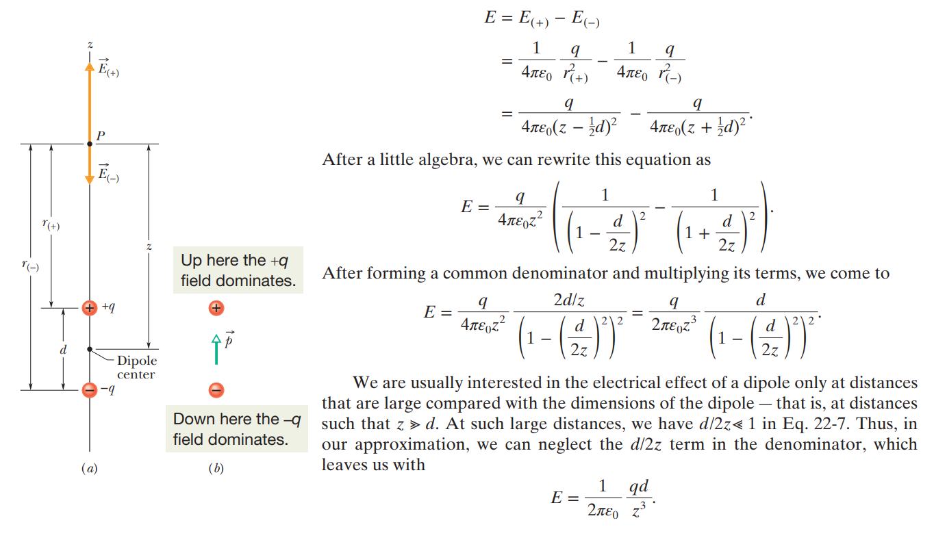
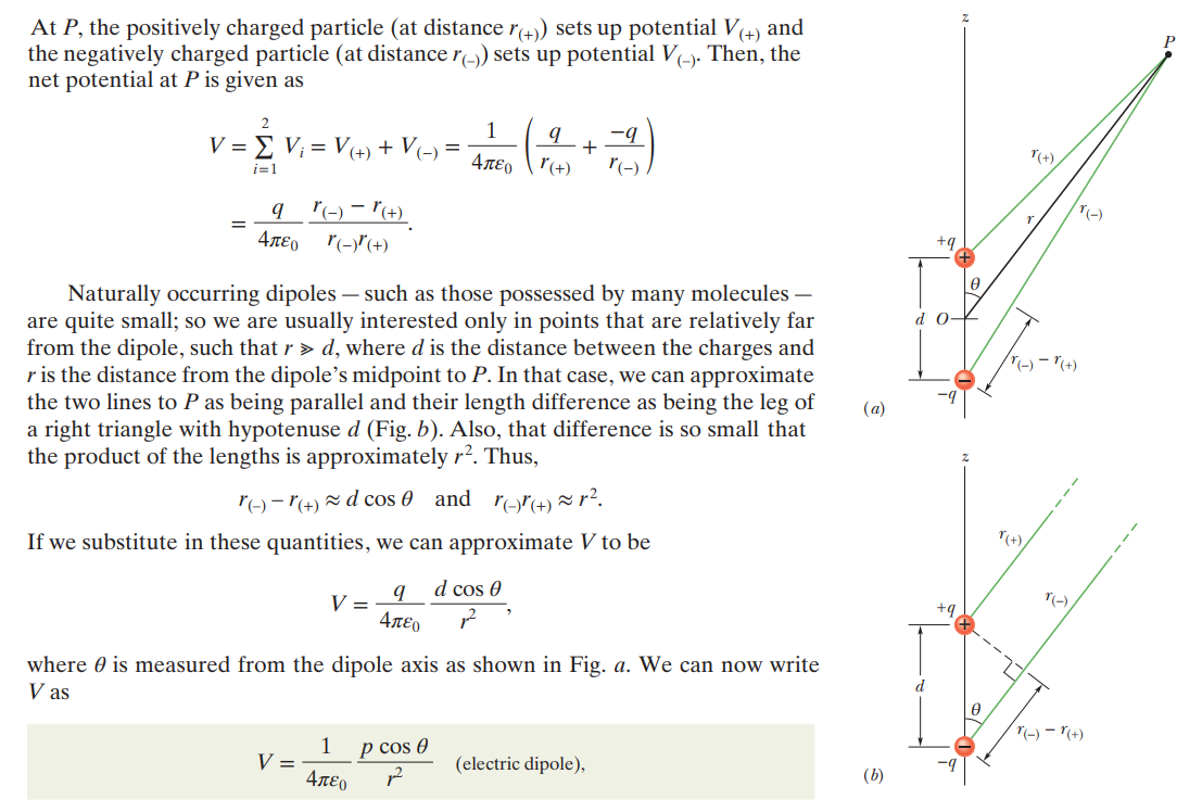