
These are my complete notes for Electric Fields in Electromagnetism.
I color-coded my notes according to their meaning - for a complete reference for each type of note, see here (also available in the sidebar). All of the knowledge present in these notes has been filtered through my personal explanations for them, the result of my attempts to understand and study them from my classes and online courses. In the unlikely event there are any egregious errors, contact me at jdlacabe@berkeley.edu.
Summary of Electric Fields (Electromagnetism)
Table Of Contents
XIII. Electric Fields.
XIII.I Introduction to Fields.
If the test charge is positive, then it will be in the same direction as the electric field, and if it is negative, then it will be in the opposite direction of the electric field. By convention, positive test charges are used to define electric fields.
#
P. Rule .
Electric Field: VECTOR.
Units: Newtons / Coulombs.
Equation:
E = (Fe / q)
E = The magnitude of the electric field at a particular point.
Fe = The electric force being felt by the charge at the particular point being measured.
q = The magnitude of the charge/charged particle of the particular point being measured.
Definition: An Electric Field is a field in space surrounding a charged object, in which the object's electric force has strength.
Electric fields have their direction expressed in the form of lines, the nature of which is elucidated in Rule 174. Naturally (meaning without the interference of another electric field), these lines, which originate at every point of the object's surface, will be perpendicular to the object and will point radially outward or inward (depending on the charge sign) forever without bending - the electric field of a point charge, for example, will shoot off in every direction in such a way. The direction and lines themselves, however, can be influenced as a result of the Law of Charges and can bend accordingly - see Rule 174.
Technically, the given equation dictates that the electric field is the "amount of electric force per charge at a point in space", the ratio between the electric force of the charge and the magnitude of the charge itself. All charge creates an electric field in relation to its electric force.
The reason an exact magnitude value can be determined for an electric field (an inherently emanating and changing entity), as is done in the given equation, is because the magnitude being found is that of the strength of electric field at a particular point, denoted by the electric force experienced by the charge placed at that point.
# Uniform Electric Field: An electric field that has the same magnitude and direction at every point within the field - think of the electric field created by an infinitely long pole. These electric fields, of course, are overtly idealized.
#
P. Rule .
The magnitude of the electric field will decrease as the test charge gets farther from the point charge, as a result of the Law of Electric Force (since the denominator distance value increases and all). The electric field surrounding (and caused by) a point charge is constant at a constant radius from the point charge.
The entire Law of Electric Force equation can be substituted into the Electric Field equation, enabling one to simplify things considerably if the circumstances allow.
The entire Law of Electric Force equation can be substituted into the Electric Field equation, enabling one to simplify things considerably if the circumstances allow.
#
P. Rule .
Electric Field Lines:
1. The lines of attraction in an electric field always point away from the positive charge (origination) and toward the negative charge (termination). Thus, the lines always point in the direction in which the test charge would experience an electric force.
2. The # of electric field lines per unit area is proportional to the electric field strength. Therefore, a higher density of electric field lines means a higher electric field strength.
3. Electric field lines always start perpendicularly to the surface of the charge, and start on a positive charge and end on a negative charge (unless there is more of one charge, in which case some lines would start/end infinitely far away).
4. Electric field lines never cross.
Use the test charge (a positive entity - see the definition) as the sample particle, for the sake of illustrating this point.
When the test charge (standardized as positive) is placed in the field of a positive point charge, the test charge will be repelled from the point charge. Electric force projects radially outward from the positive point charge, decreasing in magnitude as distance increases.
On the flip side, if the point charge is negative, then the test charge will be attracted toward the point charge. All of the arrows will point radially inward toward the negative point charge.
XIII.II Continuous Charge Distributions.
λ = (Q / L)
λ = (Lambda) The direction and magnitude of the given expression, defined in Coulombs per Meter (C / m).
Q = The charge of the object.
L = The length of the object - this form of density is best applied to charge along a flat line.
Treat λ as a constant when taking the derivative. Note, however, that the given equation can be transmuted into a derivative form: λ = (dQ / dL). This is because the ratio remains the same: total charge divided by total length is equal to the infinitesimally small individual charge over the length thereof.
# Surface Charge Density:
σ = (Q / A)
σ = (Sigma) The direction and magnitude of the given expression, defined in Coulombs per Meter Squared (C / m²).
Q = The charge of the object.
A = The total area of the object.
Treat σ as a constant when taking the derivative. Note, however, that the given equation can be transmuted into a derivative form: σ = (dQ / dA). This is because the ratio remains the same: total charge divided by total area is equal to the infinitesimally small individual charge over the area thereof.
# Volumetric Charge Density:
ρ = (Q / V)
ρ = (Rho) The direction and magnitude of the given expression, defined in Coulombs per Meter Cubed (C / m³).
Q = The charge of the object.
V = The total volume of the object.
Treat ρ as a constant when taking the derivative. Note, however, that the given equation can be transmuted into a derivative form: ρ = (dQ / dV). This is because the ratio remains the same: total charge divided by total volume is equal to the infinitesimally small individual charge over the volume thereof.
#
P. Rule .
Electric Field of a Continuous Charge Distribution (CCD): VECTOR.
Units: Newtons / Coulombs. It is a type of electric field.
Equation:
$$E_{CCD} = k \int \frac{dq}{r^2} \hat{r}$$
ECCD = The electric field that exists around a continuous charge distribution, calculated at point r in space.
k = The Coulomb constant, equal to 8.99 × 10⁹ (N × m²) / (C²).
dq = The infinitesimally small point charges, of which there is an infinite number of. This value can be substituted for any of the equivalent charge density derivatives (see Linear, Surface, and Volumetric), pursuant to the nature of a particular problem.
r = The distance between the infinitesimal charge dq and the point where the electric field is being calculated. Unlike the Law of Electric Force, this r is a function that varies depending on the charge, since there is technically an infinite number of charges (dq).
r̂ = The unit vector pointing from dq (whichever charge) toward the test charge - this is most applicable post-integral, when you can have a test charge to calculate the strength of the electric field with respect to. The direction points radially outward for positive dq, and inward for negative dq.
Definition: A Continuous Charge Distribution (CCD) is a simple concept that elaborates the simple 'point' model of charges into one that uses calculus to account for more chargetype possibilities, furthering the infinite journey into human knowledge.
A 'continuous charge distribution' is simply a charge that isn't a point charge; e.g., a charge with a shape and an electric charge continuously distributed throughout the object.
The electric field that exists around a continuous charge distribution can be determined through a rethinking of the standard Electric Field-Law of Electric Force combined equation (see Rule 172) using Calculus. Since the charged object is made up of an infinite number of infinitesimally small point charges ('dq' representing them individually), the therefore infinite number of electric fields can be calculated using an integral.
There are very specific use cases for this integral: it is not applicable everywhere. See Rule 176 for a detailed treatise on this cases and their exceptions. The limits of integration of the integral are specific to each problem and can be determined through ingenuity and through the power of the indomitable human spirit.
That pesky 'dq' thing can be switched out by taking the derivative of any of the charge densities (see linear, surface, and volumetric), depending on what one is looking for.
The Electric Potential created by a CCD has a near identical equation to its electric field, described in Rule 206.
#
P. Rule .
The integral equation for CCDs (continuous charge distributions, see Rule 175) is only applicable when every infinitesimal charge has its electric field pointing in the same direction when it is pointing toward the test point. For example: when the CCD is a flat line, and the test charge is on its same axis.
There are some workarounds in which the above stipulation is technically still respected, allowing the integral to still be used even for shapes like rings. This is when all components in all other directions cancel out, leaving only the components in a specific direction. For example, in a uniformly charged ring, the horizontal components of the field from symmetric charge elements cancel, leaving only the vertical (axial) component.
When all fails, and the direction of the electric at test charge P is simply not the same for every charge dq on the ring, then take the derivative of both sides of the equation (giving dE) and try to see if any components cancel eachother out anywhere - in order to find the components, use the direction of the electric field from or toward the test charge (remember: the direction points radially outward for positive dq, and inward for negative dq), and imagine that beyond the test charge or dq, wherever the direction points, the direction line continues - this extended line segment represents dE, which can then be broken into components (which will hopefully cancel out in one direction). If there are equal negative and positive dq's in a particular direction, then it cancels out. Ideally, the direction that doesn't cancel out should only a single sign no matter the direction/origin of the dq.
Generally, the dq electric field values in a particular direction 'cancelling out' is the result of a symmetry created by the placement of the point charge. For example, a point charge placed somewhere along the axis of the center of the ring.
If one has succeeded in cancelling out, then they would be able to proceed with all the necessary moving of sines or cosines (resultant from the components) and the general transfiguration of terms dependent on the characteristics of the problem itself. After one has been able to simplfy and reduce everything into only one real variable on one side (every other symbol just being a constant), then both sides can be integrated, creating a problem-specific version of the hyper-generalized CCD integral equation (see Rule 175).
All this component business requires that there be some reference position, a known x-axis and y-axis positioning in relation to the given CCD and point charge that can be used to derive the components from.
#
P. Rule .
Note that the farther you get from a finite continuous charge distribution, the more the electric field caused by the CCD matches the electric field caused by a point charge (as in, the simplified Law of Electric Force + Electric Force equation from way back when (see Rule 173)). Of course, this requires the distance between the test charge and the CCD to be much much greater than the internal distance with the CCD itself.
#
P. Rule .
Always be aware of what constants/variables are much much greater than others. In end game integrals, such as in CCD-type problems (see Rule 176), this can totally simplify whole entire parts of your equation by just thinking of the lesser variable as zero (where it is left alone and not acting as a coefficient). Of course, this mandates the usage of the approximation symbol (≈) for your answer.
#
P. Rule .
You can never assume that the equation for the electric field of a shape, whether 2d or 3d, will be the same if the shape is a conductor or a nonconductor. The world is not such a simple, idealistic place, even in what is essentially toy model physics (classical electromagnetism).
The key factor in determining whether the electric field equation for a shape is the same or differing between conductors and nonconductors, is how the charge distributes within the shape.
The following characteristics are indicative of identical equations between the electric field equations of a conductor and nonconductor shape:
The following characteristics are indicative of differing equations between the electric field equations of a conductor and nonconductor shape:
The key factor in determining whether the electric field equation for a shape is the same or differing between conductors and nonconductors, is how the charge distributes within the shape.
The following characteristics are indicative of identical equations between the electric field equations of a conductor and nonconductor shape:
- Infinite Reach: If the shape is infinite (like infinite planes or cylinders), then both conductors and nonconductors produce the same electric field at points sufficiently far from the charge distribution. Example: Infinite planes as explained in Rule 180.
- Symmetric Charge Distributions: There are cases in which some form of symmetry causes the charge distribution to remain unchanged between the conductor and nonconductor.
For example: an infinite line of charge with uniform charge density λ produced the same radial field for both conductors and nonconductors, since, being a line, the charge is "on the surface" regardless of the conductivity of the shape (in terms of how the charge being on the surface is an important distinction between conductors and nonconductors and alters the calculation of their electric fields - see Rule 170), and is emanating outward in the same fashion. - External Field Only: If only the electric field outside of an enclosed shape is being considered, then IF SYMMETRY DICTATES A FIXED CHARGE DISTRIBUTION (like shells and spheres and cylinders and whatnot, not just any wack enclosed shape), then the equation for that electrical field in particular will be the same whether the shape material is a conductor or nonconductor. This is more due to the first shell theorem (see Rule 171) than anything.
The following characteristics are indicative of differing equations between the electric field equations of a conductor and nonconductor shape:
- Internal Charge within Enclosed Shapes: As everyone knows, the charge within an enclosed shape for conductors and nonconductors differs as a result of charge placement in the solid part of the shape (like the shell part of a hollow shell) - see Rule 170. Conductors have zero electric field within themselves, and nonconductors do have some.
- Non-Uniform Charge Distribution: Conductors force charge to redistribute, whereas insulators allow charge to remain fixed. For example: a finite conducting "slab" (like a brick) with excess charge will concentrate charge at the edges, while a nonconductor could have uniform volume charge density.
This will cause differing internal and external electric fields, both for the reason outlined in Difference Characteristic #1 (directly above) and for not meeting the symmetricality requirement of Equivalence Characteristic #3 (further above).
#
P. Rule .
Flat Disks & Infinite Planes: VECTORS.
Units: Newtons / Coulombs. They are types of electric fields.
Equation:
$$E_{disk} = \frac{\sigma}{2\varepsilon_0} \left( 1 - \frac{z}{\sqrt{z^2 + R^2}} \right)$$ $$E_{plane} = \frac{\sigma}{2\varepsilon_0}$$
Edisk = The magnitude of the electric field produced by a uniformly charged flat disk, calculated at some point z from the central axis of said disk.
Eplane = The magnitude of the electric field of an infinite plane, independent of distance from the plane (interestingly).
σ = Surface charge density. See treatise here.
ε0 = The Permittivity of Free Space, equal to 8.85 × 10⁻¹² (C²) / (N × m²).
z = The distance (along the central axis) between the point at which the electric field is being measured, and the center of the disk. z ≥ 0.
R = The radius of the disk.
Definition: The Electric Field due to a (flat) uniformly charged disk and due to an infinite sheet are, in fact, closely related, the latter effectively being derived from the former.
The first equation gives the electric field magnitude on the central axis through a flat, circular, uniformly charged disk. The equation is derived in a highly logical and annoying manner, found here (offsite).
If one were to plug in infinity for R, letting the radius rise to infinity while keeping the z value finite, then the equation would simplify to that of the equation for the electric field of an infinite plane, the second given equation. By their very nature, all fields produced by infinite planes will be uniform, and thus will not change with respect to distance. The straight, parallel field lines will neither converge nor diverge from their source (the plane), and as such the field intensity will never change. READ: Electric Field is Uniform when created by a plane.
Note that despite the equation specifically being for disks and circular 2d shapes, the very act of making the radius infinite will create a plane, and thus makes its circular origins irrelevant.
By virtue of the shape being infinite (passing Equivalence Characteristic #1, see Rule 179), the infinite plane equation is true for both conductor and nonconductor infinite planes. Furthermore, know that it is also the equation for the electric field at the surface of a nonconductor, as explained in Rule 197.
XIII.III Dipole Moment.
#
P. Rule .
Electric Dipole, Electric Field (along dipole axis): VECTOR.
Units: Newtons / Coulombs. It is a type of electric field.
Equation:
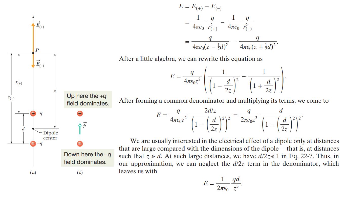
Edipole = (1 / 2πε0) × (qd / z³)
Edipole = The electric field produced by a dipole along its axis, calculated with respect to the distance between the test charge and the dipole midpoint.
ε0 = The Permittivity of Free Space, equal to 8.85 × 10⁻¹² (C²) / (N × m²).
q = The absolute value of the charge of either particle.
d = The distance between the particles.
z = The distance between the test charge (the point at which the electric field is being calculated, which, being somewhere on the dipole axis, will be directly above or below the particles) and the dipole midpoint (d/2). z MUST be >>> to d, for reasons detailed in the proof (see below).
Definition: An Electric Dipole is an arrangement of two particles (point charges) with equal charge magnitudes but opposite signs. The particles are separated by distance d and lie along the dipole axis, an axis of symmetry going through both particles.
A simple graphic of what this entails is seen below:
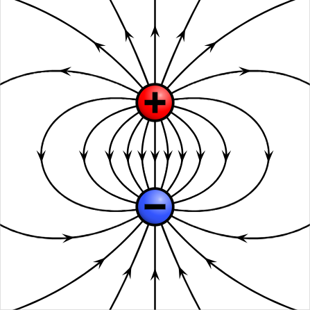 An example dipole moment, with the dipole axis running straight through the center.
The equation for the electric field produced by a dipole along its axis (and NOWHERE ELSE) is presented above. The electric field created at other points involves much more difficult, graduate-level math (offsite), and thus is dealt with much later in Physics (see Rule [[[).
There is a simple proof of the given equation, done through finding the strength of the net electric field produced by the two particles at an arbitrary point P (the test charge) along the dipole axis. It can be found here (onsite).
The internal force on the electric dipole (Fnet) will equal to zero, since the attractive forces between the particles are equal and opposite in magnitude, forming a Newton's Third Law Force Pair. They will thus be in equilibrium.
The product qd on the right side of the equation is known as the "electric dipole moment", a concept discussed in Rule 183.
The electric potential produced by an electric dipole, which can be easily found for any point (not just axial points), is detailed in Rule 205.
Units: Newtons / Coulombs. It is a type of electric field.
Equation:
Edipole = (1 / 2πε0) × (qd / z³)
Edipole = The electric field produced by a dipole along its axis, calculated with respect to the distance between the test charge and the dipole midpoint.
ε0 = The Permittivity of Free Space, equal to 8.85 × 10⁻¹² (C²) / (N × m²).
q = The absolute value of the charge of either particle.
d = The distance between the particles.
z = The distance between the test charge (the point at which the electric field is being calculated, which, being somewhere on the dipole axis, will be directly above or below the particles) and the dipole midpoint (d/2). z MUST be >>> to d, for reasons detailed in the proof (see below).
Definition: An Electric Dipole is an arrangement of two particles (point charges) with equal charge magnitudes but opposite signs. The particles are separated by distance d and lie along the dipole axis, an axis of symmetry going through both particles.
A simple graphic of what this entails is seen below:
The equation for the electric field produced by a dipole along its axis (and NOWHERE ELSE) is presented above. The electric field created at other points involves much more difficult, graduate-level math (offsite), and thus is dealt with much later in Physics (see Rule [[[).
There is a simple proof of the given equation, done through finding the strength of the net electric field produced by the two particles at an arbitrary point P (the test charge) along the dipole axis. It can be found here (onsite).
The internal force on the electric dipole (Fnet) will equal to zero, since the attractive forces between the particles are equal and opposite in magnitude, forming a Newton's Third Law Force Pair. They will thus be in equilibrium.
The product qd on the right side of the equation is known as the "electric dipole moment", a concept discussed in Rule 183.
The electric potential produced by an electric dipole, which can be easily found for any point (not just axial points), is detailed in Rule 205.
#
P. Rule .
Because of the 1/z³ dependence, the field magnitude of an electric dipole decreases more rapidly with distance than the field magnitude of either of the individual charges forming the dipole (which depends on 1/r²). Even beyond that, this is relatively clear when considering how at distant points, the electric fields of the oppositely charged particles will increasingly cancel eachother out.
#
P. Rule .
Electric Dipole Moment:
The 'qd' from the Dipole Electric Field equation (see Rule 181) is known as the Electric Dipole Moment, and can have the value 'p' substituted in for it. It has the unit of the coulomb-meter, of course.
The Dipole Moment is defined as the magnitude of the dipole, purely a matter of charge and distance. This is separate from the magnitude of the electric field of the dipole at a point - that already has its own equation established, see Rule 181. The electric field generated by the dipole is proportional to the dipole moment, though they are always in opposite directions, since the electric field points from the positive charge to the negative charge.
The Electric Dipole Moment is to the Dipole Electric Field equation, what the Discriminant is to the Quadratic Formula (see Math Rule 33), perhaps even to a further degree in which the electric dipole moment can be considered even more important than its forebear.
The direction of p is simply the axis on which the dipole resides, while the sense (see Math Rule [[[) is pointing from the negative toward the positive charge of the dipole.
# Induced Dipole Moments:
Many molecules, such as water, have permanent electric dipole moments. In all isolated atoms and in some types of molecules, the centers of the positive and negative charges coincide and thus have no dipole. These are known as nonpolar molecules.
However, if such an atom or a nonpolar molecule were to be placed in an external electric field, the field would distort the electron orbits and separate the centers of positive and negative charge, effectively creating an electric dipole.
Because the electrons are negatively charged, they tend to be shifted in a direction opposite the field. This shift sets up a dipole moment p (see Rule 183) that points in the direction of the field. This dipole moment is said to be induced by the field, while the atom or molecule is then said to be polarized by the field (that is, it has a positive side and a negative side).
When the field is removed, the induced dipole moment and the polarization disappear.

