These are my complete notes for Differential Calculus, covering such topics as Limits, Squeeze Theorem, Velocity, Acceleration, and Position, the Power Rule, Chain Rule, Quotient Rule, Particle Motion, Continuity, Optimization, Related Rates, and more.
I color-coded my notes according to their meaning - for a complete reference for each type of note, see here (also available in the sidebar). All of the knowledge present in these notes has been filtered through my personal explanations for them, the result of my attempts to understand and study them from my classes and online courses. In the unlikely event there are any egregious errors, contact me at jdlacabe@berkeley.edu.
Summary of Differential Calculus (Complete)
?. Limits.
# Average Rates/Speed: Average Speed is found by dividing the distance covered by the elapsed time.
# Limit: The value a function approaches as it becomes closer to a specified point - thus, not necessarily actually being at that point, but rather as close to it as possible with being on it. If a function is continuous near that point, the limit equals the function's value; otherwise, it will describe the behavior of the function even if undefined at that point.
# Properties of Limits:
Similar to Logarithms, Limits have their internal rules that can applied at any time. For the "commandments" version of this list, see Rule 110.
1. The limit of a constant is equal to a constant. $$\lim_{x \to a} c = c$$
2. The limit of x as x approaches a, equals a. $$\lim_{x \to a} x = a$$
3. The limit of a sum is the sum of the limits. $$\lim_{x \to a} (f(x) + g(x)) = \lim_{x \to a} f(x) + \lim_{x \to a} g(x)$$
4. The limit of a difference is the difference of the limits. $$\lim_{x \to a} (f(x) - g(x)) = \lim_{x \to a} f(x) - \lim_{x \to a} g(x)$$
5. The limit of a constant times a function is the constant times to limit of the function. $$\lim_{x \to a} [c × f(x)] = c \lim_{x \to a} f(x)$$
6. The limit of a product is the product of the limits. $$\lim_{x \to a} (f(x) × g(x)) = \lim_{x \to a} f(x) × \lim_{x \to a} g(x)$$
7. The limit of a quotient is the quotient of the limits, provided the denominator does not equal zero. $$\lim_{x \to a} \frac{f(x)}{g(x)} = \frac{\lim_{x \to a} f(x)}{\lim_{x \to a} g(x)}$$
8. The limit of a sum is the sum of the limits. $$\lim_{x \to a} (f(x))^n = (\lim_{x \to a} f(x))^n$$
#
Rule .
The average rate of change IS the slope. The average speed is the distance covered divided by the elapsed time, like miles per hour. Rate of increase is also just the derivative. First rate is first derivative, rate of the rate is second derivative, etc.
#
Rule .
Say that 16t² is the free fall motion of an object with no air resistance. It will follow the same (∆y / ∆t) formula as the slope formula.
∆ (Delta) means as "the change in", so (change in distance / change in time). From 0 to 2 seconds, the rock will travel (6(2)² - (6(0)^2)) / (2 - 0), or 34 ft/sec average speed.
∆ (Delta) means as "the change in", so (change in distance / change in time). From 0 to 2 seconds, the rock will travel (6(2)² - (6(0)^2)) / (2 - 0), or 34 ft/sec average speed.
#
Rule .
To find the instaneous speed/rate of change, the limit formula is as follows:
$$\lim_{h \to 0} \frac{f(a + h) - f(a)}{h}$$
You know a and the equation at first, plug in (a + h) to the equation and complete formula. Then, plug in 0 for h to find instantaneous velocity/speed.
#
Rule .
Speed is the time rate at which an object is moving along a path, while velocity is the rate and direction of an object's movement.
#
Rule .
There are nine holy truths of limits that must always be remembered and and held immutable. They are similar to the mystical factoring rules, and some are versions of the Limit Properties referenced previously:
- The equivalance of constants. (L.P. #1)
- The equivalance of a to x approaching a. (L.P. #2)
- The Sum Rule. (L.P. #3)
- The Difference Rule. (L.P. #4)
- The Constant Multiplication Rule. (L.P. #5)
- The Limit Product Rule. (L.P. #6)
- The Limit Quotient Rule. (L.P. #7)
- The Limit Power Rule. (L.P. #8)
- The Radical Rule. (a synthesis of L.P. #8 & #7 or #6)
#
Rule .
The one-sided limit is allowed to be infinity, while two-sided limits cannot be infinity and must not be a number.
#
Rule .
The Squeeze Theorem:
When the limit can't be found directly, find it indirectly using the squeeze theorem. The way this theorem works, is to 'squeeze' function f (which has the uncertain limit) between two functions, h and g, and find their limits. Definitionally, this is written as follows:
If g(x) ≤ f(x) ≤ h(x), where x ≠ c in some interval around c, then: $$\lim_{x \to c} g(x) = \lim_{x \to c} h(x) = L$$
The classic example of a function that must use the Squeeze Theorem is one that oscillates, such as x² × sin(1/x).
 The demonstration of how the squeeze theorem may work on a function f, with the functions h and g above and below 'squeezing' the position of f at a point, thus requiring the limit of f to match that of h and g at that point. Courtesy of Cooper's Calculus.
The key idea of the Squeeze Theorem is that if h(x), which is above f(x), has its limit at c with the same y-value as g(x), then f(x) would also have to have that limit because it is between g(x) and h(x).
When the limit can't be found directly, find it indirectly using the squeeze theorem. The way this theorem works, is to 'squeeze' function f (which has the uncertain limit) between two functions, h and g, and find their limits. Definitionally, this is written as follows:
If g(x) ≤ f(x) ≤ h(x), where x ≠ c in some interval around c, then: $$\lim_{x \to c} g(x) = \lim_{x \to c} h(x) = L$$
The classic example of a function that must use the Squeeze Theorem is one that oscillates, such as x² × sin(1/x).
The key idea of the Squeeze Theorem is that if h(x), which is above f(x), has its limit at c with the same y-value as g(x), then f(x) would also have to have that limit because it is between g(x) and h(x).
# Infinity/∞: The term 'infinity' does not refer - it describes the behavior of a function. Infinity means an increasing distance forever.
#
Rule .
The squeeze theorem also works for infinite limits.
#
Rule .
To find the horizontal asymptote, you can take the biggest thing on top, and divide it by the biggest thing on the bottom, or you could factor out the biggest base (with exponent), even if it makes every divisor weird. Then, factor to find the vertical asymptote, just plug in zero for the bottom, or cheat by using a graph.
#
Rule .
End Behavior Models
You can determine the end behavior of a complicated polynomial by looking at a similar one that acts exactly the same for extremely large values of x. For all polynomials, g(x) = an × xⁿ is the end behavior.
The function g must be:
a) A right end behavior model for f if $$\lim_{x \to ∞} \frac{f(x)}{g(x)} = 1$$
b) a left end behavior model for f if $$\lim_{x \to -∞} \frac{f(x)}{g(x)} = 1$$
#
Rule .
If the EBM is a constant, then it is a horizontal asymptote.
#
Rule .
A function's right & left end behavior models are not always the same function.
#
Rule .
Tradition dictates that for an equation with only two polynomials, the left one is the REBM and the right is the LEBM. Yes, opposite of what one may immediately think.
# Reciprocal Substitution:
There is a very specific and unique characteristic of Limits that must always be kept in mind when performing problems. Reciprocal substitution can be performed by taking the variable of the limit (90% of the time being x), flip it to its reciprocal (e.g., 1/x for x), and switch the term of the limit as shown below. This reciprocal is performed even for x's inside of trig. functions - it is done for all instances.
$$\lim_{x \to ∞} \frac{1}{x} = \lim_{x \to 0^+} x$$ $$\lim_{x \to -∞} \frac{1}{x} = \lim_{x \to 0^-} x$$
Infinity goes to Zero-Right, as Negative Infinity goes to Zero-Left. The nature of the reciprocal is not specific a specific side - either infinity or the zero could have 1/x or x.
#
Rule .
Rampant idiocracy has softened testing policy enough that you may be able to, in essence, cheat and look at the graph to determine values like the end behavior mode and asymptotes.
#
Rule .
If the assumed number for the LEDM of some two-polynomialed equation doesn't work, then try the answer for the REBM. Same for the issue vice-versa.
#
Rule .
For piecewise functions, even if x is ≥ or ≤ or > or whatever to 0, a (Lim x→0⁻) will make the function go to the f(x) for less than zero, and (Lim x→0⁺) makes it go to x > 0. Think of it like the plus and negative signs -0.1 or add 0.1 to the value.
?. Continuity.
#
Rule .
Any function y = f(x) whose graph y = f(x) can be sketched in one continuous motion without lifting the pencil is an example of a continuous function.
#
Rule .
There are two RULES of CONTINUITY, which if both met, establish UNIVERSAL CONTINUITY for a function.
- A function y = f(x) is continuous at an inerior point c of its domain if:
$$\lim_{x \to c^-} f(x) = \lim_{x \to c^+} f(x) = f(c)$$ $$\lim_{x \to c} f(x) = f(c)$$ - A function y = f(x) is continuous at a left endpoint a if:
$$\lim_{x \to a^+} f(x) = f(a)$$ and is continous at a right endpoint b of its domain if: $$\lim_{x \to b^-} f(x) = f(b)$$ If a function f is not continuous at a point x, we say that f is discontinuous at c, and that c is a "point of discontinuity" of f.
#
Rule .
Continuous Function are continuous everywhere on their domains. Properties of Continuous Functions f & g are continuous at x = c.
All polynomial and Radical functions are continuous everywhere with no Points of Discontinuities. On the other hand, all rational and trig. functions are only continuous along their domain; they have Points of Discontinuities wherever the denominator equals 0.
All polynomial and Radical functions are continuous everywhere with no Points of Discontinuities. On the other hand, all rational and trig. functions are only continuous along their domain; they have Points of Discontinuities wherever the denominator equals 0.
# Operation Terminology Refresher:
- Sums: f + g
- Differences: f - g
- Products: f × g
- Constant Multiples: k × f, where k = any real #.
- Quotients: f/g, g ≠ 0.
#
Rule .
If f is continuous at c, and g is continuous at f(c), then the composite g ∘ f is continuous at c.
#
Rule .
A function is continuous even if it has Points of Discontinuity, as long as these points are not within the domain. For example, 1/x is considered to be continuous along its domain, despite the absurdity of its graph.
#
Rule .
A function passes the Intermediate value theorem if it never takes on two values without taking on every value in between. A continuous function f on a closed interval [a, b] will take on every y-value between f(a) and f(b), given no discontinuities.
#
Rule .
Jump Discontinuities: Where the left & right side limits are not equal.
Infinite Discontinuities: Where the discontinuity is an asymptote.
Removable Discontinuities: A detached dot, floating on the plane, where the limit continues to be a real number.
Oscillating Discontinuities: A discontinuity that oscillates back and forth, son. Examples include sin(1/x). These functions are discontinuities because no matter how far you zoom in, it will still be oscilliating, thus lacking local linearity.
#
Rule .
For Discontinuities: Jump beats hole. Infinite beats Jump. Oscillating is in a league of its own, as it can only be sin(1/x) or something of the sort.
?. Derivatives.
#
Rule .
A secant line is a line that intersects the line at two places. The slope of the secant line is the average rate of change between the two points.
#
Rule .
A tangent line is a line that intersects a curve at exactly one point. The slope of the tangent line is the instantaneous rate of change at a point.
# Difference Quotient: $$\frac{f(x + h) - f(x)}{h}$$ The "Difference Quotient", given above, represents the secant line of a curve from the point (a, f(a)) to (a+h, f(a+h)), which is also the average rate of change from x=a to x=a+h:
# Normal Line: The line normal to a curve is the line perpendicular to the tangent at that point.
#
Rule .
When the limit exists, it's called the derivative of f at a, or any point. The derivative is f'(x) =
$$\lim_{h \to 0} \frac{f(x + h) - f(x)}{h}$$
provided the limit exists. "Differentiate" means to determine the Derivative.
# Verbal Descriptions of Calculus Notation:
#
Rule .
Graphing the derivative without knowledge of the formulas for dy/dx nor the parent function, is wack:
First, get the slope between two points on the original f(x) and find the slope. As x increases, a decreasing f(x) value indicates a negative slope, while an increasing f(x) value indicates a positive slope. Find an x-value in the middle of the two points and use it as the x-value. Use the slope as the y-value and plug into the new graph, and repeat. Fo a graph with "pointy points", known as corners, they are undefined in the derivative graph (the f'(x)), as they do not have local linearity (see [[[).
First, get the slope between two points on the original f(x) and find the slope. As x increases, a decreasing f(x) value indicates a negative slope, while an increasing f(x) value indicates a positive slope. Find an x-value in the middle of the two points and use it as the x-value. Use the slope as the y-value and plug into the new graph, and repeat. Fo a graph with "pointy points", known as corners, they are undefined in the derivative graph (the f'(x)), as they do not have local linearity (see [[[).
#
Rule .
When a fraction has a square root, standard procedure is to multiply it by a conjugate, especially if the square root is on the denominator.
#
Rule .
For the alternate definition of the derivative, you always want to do all the algebra first before substituting for a at the end. Then, you can do a.
#
Rule .
Function f(x) is differentiable on a closed interval [a, b] if it has a derivative at every interior point of the interval, and if the limits below exist at the endpoints.
$$\lim_{h \to 0^+} \frac{f(a + h) - f(a)}{h}$$ is the right-hand derivative, and
$$\lim_{h \to 0^-} \frac{f(b + h) - f(b)}{h}$$ is the left-hand derivative.
$$\lim_{h \to 0^+} \frac{f(a + h) - f(a)}{h}$$ is the right-hand derivative, and
$$\lim_{h \to 0^-} \frac{f(b + h) - f(b)}{h}$$ is the left-hand derivative.
#
Rule .
The left hand derivative can be found by using the regular f(x), while the right hand derivative is found by using the equation of the f'(x) derivative found from the left hand derivative. If the two derivatives are equal to each other, then the derivative in totality is real.
# Differentiability: The ability to find slope at a point, which is necessary to take the derivative.
# Cases when f'(a) doesn't exist (or, when a point is non-differentiable):
- A Corner: f(x) = |x|
A corner occurs when, at the point a, the function on the graph will make a sharp turn, and its slope will change instantaneously.
- A Cusp: f(x) = x2/3
A cusp occurs when the line gradually curves into a sharp corner. In effect, the cusp is a special case of the corner: the cusp only has one possible tangent, while a corner has two distinct ones.
- A Vertical Tangent: f(x) = ∛x
When the line is vertical, there is no slope, and thus it is non-differentiable at that point.
- A Discontinuity:
For example, a non-continuous piecewise function. The derivative (nor the limit, if it is a jump discontinuity) exists at a point that is discontinous.
# Local Linearity: If you focus on a point on a curve, if you continuously zoom in on the point, eventually the graph of the curve at the point will resemble a line. Differentiability implies local linearity.
#
Rule .
The symmetric difference quotient is as follows:
$$f'(x) = \lim_{h \to 0} \frac{f(x + h) - f(x - h)}{2h}$$
It is used any time you want the derivative from each side of the tangent line (the distance being h), rather than from just one side.
#
Rule .
A derivative is a limit. Not only does the limit have to exist, it must also be continuous. The slope on the left being different from the derivative on the right rules out corners from having derivatives. If the slope becomes a vertical line (e.g., slope/m = infinity), then the derivative also does not exist.
# General Rules of Derivatives:
- Constant Rule: (d/dx) c = 0
- Power Rule: (d/dx) xn = nxn-1
- Trigonometric Rules: (d/dx) sin(x) = cos(x)
(d/dx) cos(x) = -sin(x) - Exponential Rule: (d/dx) bx = bx × ln(b)
- Logarithmic Rule: (d/dx) ln(x) = 1/x
#
Rule .
For a derivative to be, it must have local linearity. No matter how much you zoom into a corner or cusp, they will never have local linearity, and this is why they are considered "non-differentiable" entities.
#
Rule .
When taking the derivative at zero of any function f(x) = xeven/odd, for any matching exponent value, it will never exist. xeven/odd will always produce a corner or cusp at x=0, and thus cannot have a derivative at that point.
# Theorem of Differentiability: Differentiability implies continuity. However, continuity does not imply differentiability. If f has a derivative at x = a, then f is continuous at x = a.
# Intermediate Value Theorem (for Derivatives): If a and b are any two points in an interval on which f is differentiable, the f' takes on every value between f'(a) and f'(b).
#
Rule .
Laws of Differentiation
As used below, all functions f(x), g(x), and h(x), are differentiable functions, and n & c are constants.
As used below, all functions f(x), g(x), and h(x), are differentiable functions, and n & c are constants.
- Law 1: Derivative of a Constant.
f(x) = c
c ∈ ℝ
f'(x) = 0.
Examples: f(x) = 5, f'(x) = 0, slope is 0.
- Law 2: Power Rule.
f(x) = xn
f'(x) = n × xn-1
Examples: f(x) = x², f'(x) = 2x.
- Law 3: Constant Multiple Rule.
f(x) = c × h(x)
f'(x) = c × h'(x)
Examples: f'(x) = 2x³, f'(x) = 2[(x³)'], f'(x) = 6x²
f(x) = 4x⁶ + 2x10, f'(x) = 24x⁵ + 20x⁹
- Law 4: Sum and Difference Rule.
(f(x) ± g(x))' = f'(x) ± g'(x)
Examples: f(x) = 2x + x², f'(x) = 2 + 2x
#
Rule .
In order to find the horizontal tangents of a curve, you must find the derivative and then make it equal to 0, and then factor as you see fit.
# Product Rule:
(f × g)' = f'g + fg'
# Quotient Rule:
(f / g)' = (f'g - fg') / (g²)
# Higher Order Derivatives:
- y' = (dy / dx) is the first derivative of y with respect to x.
- y'' = (d²y / dx²) is the second derivative of y - double prime.
- y''' = (d³y / dx³) is the third derivative of y - triple prime.
- y(n) = (dny / dxn) is the nth derivative of y - nth prime.
#
Rule .
Derivatives are allowed to be plugged in over addition and subtraction operations, such as (d/dx)(7v - 3u), requiring the substitution of the derivatives of v and u into the equation.
#
Rule .
The derivative is the slope (rate of change) at any given point on a curve: If you are given a graph of x and asked to find the graph of the "rate of change", just find the derivative graph: The values to be plugged into the Product or Quotient rules are already given!
?. Particle Motion.
#
Rule .
If s(t) represents the position of an object, then the velocity of the object is given by v(t) = s'(t). If v'(t) represents the velocity of an object, then the object's speed is given by the absolute value of velocity. speed = |v(t)| = |s'(t)|.
# Acceleration: If v(t) represents the velocity of an object, then the acceleration of the object is given by a(t) = v'(t) = s''(t). This represents the rate at which the rate of change is changing (see Rule 147).
#
Rule .
Velocity is the speed in relation to something, so a ball can have negative and positive velocity as it is thrown in the air. Speed is just how fast it's going, and nothing can ever go negative speed.
Acceleration is the derivative of velocity, is the derivative of speed. Acceleration is positive wherever the line of the velocity graph is increasing and negative when decreasing.
Acceleration is the derivative of velocity, is the derivative of speed. Acceleration is positive wherever the line of the velocity graph is increasing and negative when decreasing.
# Fundamental Particle Motion Terms:
Displacement: S(tf) - S(ti), in effect (PositionFinal - PositionInitial)
Average Velocity: (∆S / ∆t)
Instantaneous Velocity: (ds/dt), v(t) = s'(t)
#
Rule .
Displacement is the distance between where you started from and where you ended up.
Total distance is how much distance you covered. For example, the displacement can be zero because you can end up exactly where you started.
Total distance is how much distance you covered. For example, the displacement can be zero because you can end up exactly where you started.
# Application of Calculus: Cost Modeling:
In manufacturing, the cost of production c(x) represents the cost of producing x number of units. The marginal cost is the rate of change, or "the cost to produce one more item". Marginal cost is the derivative of cost: c'(x).
Revenue, r(x) is the total amount of money collected for the sales of a product. Marginal Reveue is the total amount collected from selling one more unit. r'(x) = Marginal Revenue.
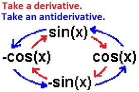
# Sine-Cosine Derivative Loop:
#
Rule .
To find when a particle is moving forward or backward, make a number line for the x's of the velocity graph and find when it is negative or positive: positive is forward, negative is backward.
For where the particle is speeding up or slowing down, if the particle has v(t) > 0 & a(t) < 0, or v(t) < 0 & a(t) > 0 (e.g., the signs do not match between the velocity and acceleration), then the particle is slowing down.
If the particle has v(t) < 0 & a(t) < 0 or v(t) > 0 & a(t) > 0 (matching signs between velocity and acceleration) then the particle is speeding up.
#
Rule .
For equations that have two functions that are just sum or difference and not product nor quotient, you can find the derivative of each individual function and continue the sum and difference as so:
f(x) = sin(x) - cos(x)
f'(x) = cos(x) + sin(x)
f(x) = sin(x) - cos(x)
f'(x) = cos(x) + sin(x)
#
Rule .
Particle Motion in a Nutshell:
Displacement: The change in position of the particle. S(tf) - S(ti)
Total Distance: The cumulative distance traveled between the starting and ending points of the particle. Found by finding every point in which the velocity changes sign, and absolute valuing all distances traveled under negative velocities while summing everything up.
Speeding up: The v(t) and a(t) of the particle have the same sign.
Slowing down: The v(t) and a(t) of the particle have differing signs.
?. Inverses.
#
Rule .
Steps for Implicit Differentiation:
- Differentiate both sides with respect to x.
- Collect the terms with dy/dx on one side of the equation.
- Factor out dy/dx.
- Solve for dy/dx.
#
Rule .
For Implicit Differentiation, only when finding the derivative of y do you need to get dy/dx and use the chain rule. For x, you can just find the derivative with the power rule.
#
Rule .
When writing powers of trigonometric functions, like y = sin³(x), always rewrite the function like y = (sin(x))³. This will make it easier to take derivatives, if needed, and is just a simpler way of seeing the exponential.
#
Rule .
To find the derivative of the inverse of a function, use the formula 1/f'(g(x)) without multiplying by the derivative of the inner function.
#
Rule .
To find the implicit differentiation of trigonometric functions, you just take the derivative of the function itself multiplied by the y': sin(y) = cos(y) × dy/dx.
#
Rule .
The inverse of the function f(x) = y is found simply by reversing the x & y values in the function. If f is differentiable at every point of an interval I, and df/dx is never zero along I, then f has an inverse and f-1 is differentiable at every point on interval f(I).
df/dx is never zero because a function only has an inverse when it is ALWAYS increasing or decreasing. ([[[must past horiz. and vert. line test]]])
df/dx = 0 means a horizontal tangent not increasing or decreasing at that point. Horizontal tangents can denote a change in direction of the function, as long as the sign of df/dx changes from before and after the found horizontal tangent point.
# Inverse Trigonometric Derivatives:
(d/dx) sin⁻¹(x) = (1 / √1 - x²) |x| < 1.
(d/dx) csc⁻¹(x) = (-1 / |x|√x² - 1) |x| > 1.
(d/dx) cos⁻¹(x) = (-1 / √1 - x²) |x| < 1.
(d/dx) sec⁻¹(x) = (1 / |x|√x² - 1) |x| > 1.
(d/dx) tan⁻¹(x) = (1 / 1 + x²) all real #s.
(d/dx) cot⁻¹(x) = (-1 / 1 + x²) all real #s.
#
Rule .
In order to find the derivative of the inverse of a function when only knowing the x-value & the function formula, plug in the x-value into the function to get the y-value, and then do 1/f'(y).
In doing so, you find the derivative of the function while plugging in the y-value under f⁻¹(x) = 1/f'(y).
In doing so, you find the derivative of the function while plugging in the y-value under f⁻¹(x) = 1/f'(y).
?. Chain Rule.
(f(g(x)))' = f'(g(x)) × g'(x)
# Integers with Exponential Powers:
For a > 0, and a ≠ 1, (au)' = au × ln(a) × (du/dx)
Without the chain rule for the exponent, this simplifies to (ax)' = ax × ln(a).
#
Rule .
(ex)1 is just ex. Whenever finding the derivative of an equation involving ex, just copy that original ex expression and multiply by the chain rule.
#
Rule .
For other expressions where x is part of the exponent, like 9-x or 3csc(x), you copy the original equation, multiply by ln of the base, and by the derivative of the exponent: 3csc(x) = ln(3) × 3csc(x) × -csc(x)cot(x). See the Integers with Exponential Powers blue section.
#
Rule .
For finding the derivative of an equation with ln, know that (ln(x))' = 1/x, with the x changing as needed. The derivative is just the changed value of 1/x multiplied by the derivative of the x-value: (ln(x²))' = (1/x²) × 2x.
#
Rule .
To find the derivative of a logarithm, for a > 0 and a ≠ 1, you must use the chain rule:
$$\frac{d}{dx} \left( \log_a x \right) = \frac{1}{x \ln(a)} \times x'$$
This means that after 1/xln(a), the chain rule would be applied for 2nd value (not the base - in this case a is the base).
Example: (log42x)' = (1 / 2xln(4)) × 2
= 1/xln(4)
It is the ln of the 1st value (the base) of the logarithm that is used.
Example: (log42x)' = (1 / 2xln(4)) × 2
= 1/xln(4)
It is the ln of the 1st value (the base) of the logarithm that is used.
#
Rule .
If you have to find the derivative of a function that requires using the chain rule to multiply by the derivative of a part of the function, and that part of the function is a constant such as ln(2) or log22, e.g. nowhere there is an x, then the derivative equals zero. eln(2), for example.
?. Extreme Values.
#
Rule .
The derivative does not exist where the function does not. The tangent line at a point represents the slope of that point, as made possible by local linearity (see definition).
#
Rule .
To find at which point of a curve the tangent line is PARALLEL to another line, just find the derivative of the first line to get the slope of the tangent line. Then, just set that derivative equal to the slope of the 2nd line. To find when a tangent line is PERPENDICULAR to another line, do the same thing except set the first line derivative equal to the negative reciprocal of the 2nd line slope.
#
Rule .
In order to find the slope of a line that passes through the origin or any other point that is tangent to a curve, you have to set 2 equations equal to eachother.
First, for example, if y = ln(x/2) and the line passes through (0,0), the slope of the line at that point will equal:
$$\text{m} = \frac{ln(\frac{x}{2})-0}{x-0} = \frac{ln(x) - ln(2)}{x}$$ Secondly, find the derivative of the curve, which is (2/x) × (1/2) or 1/x.
Finally, you set the two equations equal to eachother:
$$\frac{1}{x} = \frac{ln(x) - ln(2)}{x}$$ 1 = ln(x) - ln(2)
ln(x) = 1 + ln(2)
eln(x) = e1 + ln(2)
x = e × eln(2)
x = 2e
m = 1 / 2e
Remember to put the result back into the derivative of the equation at the end.
#
Rule .
To find the domain of a derivative, remember it conforms to the domain of the function as well. For example, if a vertical function is x ≠ 4 and x > 0, then the full domain is x > 0 and x ≠ 4.
#
Rule .
When there's an x in the base and the exponent, such as with y = xx, you have to go the long way around with the ln (or log, if that's how you want to do it) to bring down the exponent and isolate x:
ln(y) = ln(xx)
(1/y) × (dy/dx) = ln(x) + (x × 1/x)
(dy/dx) = y(ln(x) + 1)
(dy/dx) = xx(ln(x) + 1)
The same sort of thing works with trigonometric functions in the exponent.
ln(y) = ln(xx)
(1/y) × (dy/dx) = ln(x) + (x × 1/x)
(dy/dx) = y(ln(x) + 1)
(dy/dx) = xx(ln(x) + 1)
The same sort of thing works with trigonometric functions in the exponent.
#
Rule .
Steps for determining the graph of a derivative:
First, find when the graph is flat, when the curve is parallel to the x-axis. These points will be the zeroes of the derivative graph.
Remember that the derivative graph represents the speed with which the slope of the function is changing, the rate of the rate of change.
For example, the derivative graph of:
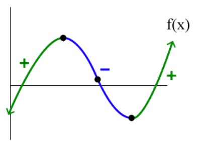 The graph of a standard function, perhaps that of a polynomial. Courtesy of Calcworkshop.
Would be:
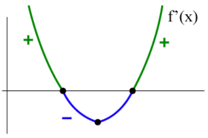 The graph of the derivative of the function given above. Courtesy of Calcworkshop.
First, find when the graph is flat, when the curve is parallel to the x-axis. These points will be the zeroes of the derivative graph.
Remember that the derivative graph represents the speed with which the slope of the function is changing, the rate of the rate of change.
For example, the derivative graph of:
Would be:
#
Rule .
Absolute (Global) Extreme Values:
Let f be a function with Domain "D". Then f(c) is the:
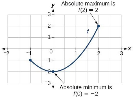 The Absolute Maximum and Absolute Minimum values for a restricted portion of a function. Courtesy of Lumen Learning.
Let f be a function with Domain "D". Then f(c) is the:
- absolute maximum value on D if & only if f(x) ≤ f(c) for all x in D. Every y-value is less than particular y-value of f(c).
- absolute minimum value on D if & only if f(x) ≥ f(c) for all x in D.
# Absolute Extrema: Average Speed is found by dividing the distance covered by the elapsed time. Consequently, there also exists relative extrema (also known as local extrema) for maximum and minimum values that are not absolutes of their function (see Rule 172).
#
Rule .
The Extreme Value Theorem:
If f is continuous on a closed interval [a, b], then f has both a minimum and a maximum value on the interval.
If f is continuous on a closed interval [a, b], then f has both a minimum and a maximum value on the interval.
#
Rule .
Local Extreme Values:
Let c be an interior point on the domain of the function f. Then, f(c) is a:
Let c be an interior point on the domain of the function f. Then, f(c) is a:
- local maximum value at c if & only if f(x) ≤ f(c) in the same interval containing c.
- local minimum value at c if & only if f(x) ≥ f(c) in some open interval containing c.
#
Rule .
Individual Local Maxes (see Rule 172) can be created by restricting the domain, same with Local Minimums. They seriously work by just looking for the highest and lowest points on the position graph (if given).
The Global Max or Min. (see Rule 170) will be the highest or lowest within the graph itself. For situations in which the probable minimum or maximum number isn't on an exact x-value, it doesn't exist because you could get infinitely close to the open point value without actually getting there in a real number.
The Global Max or Min. (see Rule 170) will be the highest or lowest within the graph itself. For situations in which the probable minimum or maximum number isn't on an exact x-value, it doesn't exist because you could get infinitely close to the open point value without actually getting there in a real number.
#
Rule .
Finding Extreme Values:
If a function has a local max or min. at an interior point c of its domain, and if f'(x) exists at c, then f'(c) = 0.
This is very obvious and should be childsplay to the novice mathematician.
If a function has a local max or min. at an interior point c of its domain, and if f'(x) exists at c, then f'(c) = 0.
This is very obvious and should be childsplay to the novice mathematician.
#
Rule .
Critical Points:
The Critical Points of a function are the points (x-values) in which the function changes from increasing to decreasing or from decreasing to increasing. There are two ways to find these points: 1., by taking the derivative of the function and finding the points at which the derivative function equals to zero, and 2. by finding the points at which the derivative function equals DNE (e.g., where the denominator of a fraction equals zero).
The first way, setting the derivative of a function equal to zero, is relatively simple. Find the derivative of the function, and then set it equal to zero and isolate x. The 'zeroes' of the function, the values that, if plugged into the x of the derivative, will produce zero, are the x-values of the critical points. To find the y-values, plug in the found x-values into the function itself (the non-derivative, original function).
For the second way, critical points also exist where f'(x) = DNE, which algebraically generally just means that the denominator of the derivative equals zero, in circumstances in which the derivative is a fraction.
For an example of the first way:
f(x) = x³ - 3x² + 2
f'(x) = 3x² - 6x = 0
3x(x - 2) = 0
x = 0 & x = 2
Thus, where f'(x) = 0 & where f'(x) = DNE is where the critical points of a function reside.
#
Rule .
To find the Extrema Points, first plug in the endpoints to the function, make a line graph with endpoints and the Critical Points, and plug in the numbers in between to find whether the Critical Point is a maximum or minumum. The endpoints can be compared to find which is the global minimum/maximum and which is the local.
Plug in the #'s into the derivative function, and the Critical Points into the regular function.
Although a function's extreme points can only exist at a function's critical points or endpoints, not every critical point or endpoint signals the presence of an extreme value. If both sides of a critical point on a line graph are positive or negative, then the critical point is not a min or max.
#
Rule .
In quadratic fractions, the numerator determines the zeroes, and the denominator determines where the function is not defined.
#
Rule .
To find the derivative of a piecewise function, just take the derivative of the equations and keep the "x > 1" stuff the same. This can be used in the same pattern as the reuglar method seen in Rule 176.
#
Rule .
Mean Value Theorem:
If y = f(x) is continuous at every point of a closed interval [a, b] and differentiable at every point of its interval (a, b), then there is atleast one point c in (a, b) at which the instantaneous rate of change equals the mean rate of change:
$$f'(x) = \frac{f(b) - f(a)}{b - a}$$
If y = f(x) is continuous at every point of a closed interval [a, b] and differentiable at every point of its interval (a, b), then there is atleast one point c in (a, b) at which the instantaneous rate of change equals the mean rate of change:
$$f'(x) = \frac{f(b) - f(a)}{b - a}$$
#
Rule .
The way to show an equation satisfies the Mean Value Theorem is to first find the y-values for the endpoints of the interval and plug them into the slope formula (Rule 179): (f(b) - f(a)) / (b - a). Then, find the derivative of the equation and set it equal to the previously found value. If it is between the endpoints, it satisfies the Mean Value Theorem.
# Antiderivative: A function F(x) is an antiderivative of a function f(x) if F'(x) = f(x) for all x in the domain of f. To find the antiderivative for the most simple functions (those that involve only a variable and its exponent, x & n), use the following equation:
$$\frac{x^{n+1}}{n+1} + C$$ The "+ c" is a value that is added to all antiderivatives, to account for the possibility that an additional constant could have been part of F(x), and that by taking the derivative, it was reduced to zero (as stated in Law 1 of the Laws of Differentiation, Rule 142). "+ c" is the degree of uncertainty of the antiderivative, and can be found through mathematical tricks learned later on (see Rule [[[)
The concept of an antiderivative will eventually evolve into that of the integral (see section [[[), which is basically just finding the antiderivatives of different functions, something that becomes surprisingly more complicated over the course of more and more difficult functions. Derivatives are extraordinarily easier.
#
Rule .
Notice that f may have local extrema at some critical points while failing to have them at others. When f has a min f' < 0 on on the left of the Critical Point, and f' > 0 on the right, there is a minimum. Vice versa for the max. If the derivative changes sign at the critical point, there is a min. or a max.
#
Rule .
For the simplified MVT proof, like the speeding trucker, you can just divide the distance by the time & say that MVT states that the average speed must equal instantaneous speed at some point.
#
Rule .
To get the antiderivative, you need to use the equation listed in the antiderivative definition (see above), with the Xn+1 / n+1 and whatnot, and then plug in the point into the antiderivative function (if known) to get c.
#
Rule .
For 'falling from rest' questions, the acceleration is generally 9.8 m/sec², given that the object is falling on Earth. And given that the object is falling from rest, v(0) = 0. However, if propelled downward, v(0) = -x, whatever specified, positive if propelled upward.
#
Rule .
Use this guide to write all explanations for finding where a function is increasing or decreasing: "Since f'(x) < 0 from (C.P., C.P.) & f'(x) > 0 from (C.P., ∞), y is a local max at x = x. Since domain is (-∞, ∞), there are no absolute extrema.
?. Derivative Tests.
Which way the graph bends or shapes, either 'up' or 'down', as defined below.
a) Concave up on an open Interval I if y' is increasing on I. This is the part of the curve on the position graph where the tangent line is on the *bottom* of the curve.
b) Concave down on an open Interval I if y' is decreasing on I. This is the part of the curve on the position graph where the tangent line is on the *top* of the curve.
# Concavity Test:
a) Concave up on any interval where y'' > 0.
b) Concave down on any interval where y'' < 0.
# Point of Inflection: A point on the graph where a tangent line exists and where the concavity changes (i.e., where the y'' changes sign).
#
Rule .
Properties of the Second Derivative (y''):
1. y'' = 0 does not always ive an inflection point. Sometimes both sides are the same sign, like in a parabola, or continually increasin or decreasing, like with x³. For example, with the function f(x) = x⁴, f'(x) = 4x³ and f''(x) = 12x². Although f''(x) = 0 at x=0, it cannot be considered an inflection point as the concavity doesn't change: f''(x) remains positive before and after.
2. y'' ≠ 0 can still be an inflection point, surprisingly. In the example f(x) = ∛x = x¹/³, f'(x) = (1/3)x⁻²/³, f''(x) = (-2 / 4∛x⁵). As evident, f''(0) is DNE, but it is also shockingly still an inflection point. An inflection point can occur where f''(x) = 0, or where f''(x) is DNE, since the only requirement is wherever f''(x) changes signs, regardless of continuity. To check, use the second derivative test.
#
Rule .
Second Derivative Test Basics:
If f'(c) = 0 and f''(c) > 0, then f has a local minimum at x = c. It should look something like the following, with the tangent line drawn in red:
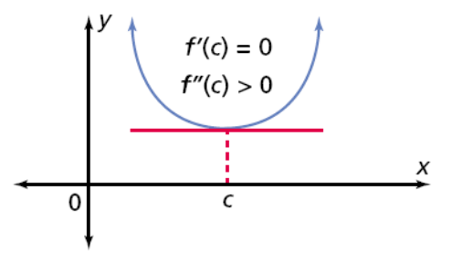 An example local minimum graph, with the first and second derivatives given and a red tangent respective to the concavity. Courtesy of Mr. Hardy's Virtual Classroom.
If f'(c) = 0 and f''(c) < 0, then f has a local maximum at x = c. It should look something like the following, with the tangent line drawn in red:
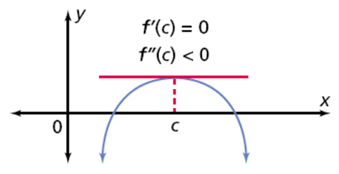 An example local maximum graph, with the first and second derivatives given and a red tangent respective to the concavity. Courtesy of Mr. Hardy's Virtual Classroom.
If f''(c) = 0 or DNE, the Second Derivative test fails. Go back & use the first derivative test. DON'T CONFUSE THE CONCAVITY TEST (see blue sec.) WITH THE SECOND DERIVATIVE TEST!!!!!!
If f'(c) = 0 and f''(c) > 0, then f has a local minimum at x = c. It should look something like the following, with the tangent line drawn in red:
If f'(c) = 0 and f''(c) < 0, then f has a local maximum at x = c. It should look something like the following, with the tangent line drawn in red:
If f''(c) = 0 or DNE, the Second Derivative test fails. Go back & use the first derivative test. DON'T CONFUSE THE CONCAVITY TEST (see blue sec.) WITH THE SECOND DERIVATIVE TEST!!!!!!
#
Rule .
First Derivative Test:
The first derivative test is used to find a graph's local minimum and maximum using the first derivative: to find these values, the points at which f is increasing and decreasing must be determined, which can luckily be found from the critical points on the derivative graph - the points at which f'(x) = 0 or DNE.
On the derivative, if f'(x) changes signs from positive to negative at c, then f has a local maximum. Vice verse for local minimums.
VERY IMPORTANT: Where f'(x) doesn't change sign, there are no extreme values. The endpoints are almost always extreme values because the graph generally increases or decreases right after them. To circumvent using the sign chart, just do the math before and after the Critical Points to find where it is increasing or decreasing and write, for example, "local max at x = -2 because f'(x) changes sign from + to -".
Remember that the sign going from positive to negative means a local maximum because that means a peak. When it goes from negative to positive, that is a minimum because it is a nadir.
#
Rule .
Graphing Functions using Derivative Tests:
To graph a function, you need to know how the graph bends along its domain, which is to say its concavity(s). Where the graph has a tangent line along the bottom of the graph, it is concave up, and when the tangent line is on top, the graph is concave down. The graph is concave up when y' is increasing, or when y'' > 0, and vice verse for concave down.
To find the concavity, you have to find the Points of Inflection, or the points where f''(x) = 0 or DNE. These are like the 2nd derivative's own Critical Points. You find them by finding the points at which the 2nd derivative is equal to 0 or DNE, and then plugging in the values on either side to see if the 2nd derivative changes sign. From there, each interval of the graph that f''(x) is positive is concave up, and each that is negative is concave down, so you can write something to the effect of "concave up from (0,2) because f'(x) is positive along that interval" for your statement.
#
Rule .
There is a neat trick to check the minimums and maximums found in the first derivative test using the 2nd derivative. It allows you to avoid having to find the signs of the values around the Critical Points in the first derivative.
Only if f'(c) = 0 and f''(c) < 0 can f have a local maximum at x = c. Only if f(c) = 0 & f'(c) > 0 does f have a local minimum at x = c.
For example, if you get a Critical Point of -2 and the f'(x) = 6x, you can immediately know that x = -2 is a local maximum because the f''(c) is -12. Yes, it's backwards.
#
Rule .
DERIVATIVE TEST SUMMARY:
IN SUMMARY: The first derivative will tell us the minimums and the maximums, the critical points, and where the graph is increasing and decreasing. The second derivative will tell us the points of inflection and the concavity, as well as enabling a trick for the minimums & maximums. To find the intervals in which f is increasing, you need the first derivative and to find the points in between the Critical Points to plug into said derivative to see what intervals the graph is facing up, you need to know the 2nd derivative & the points of inflection, finding the points in between and plugging them in as before to find what intervals are positive and thus concave up.
To find what x-coordinates have local extrema, you use the same Critical Point from finding the increasing and decreasing intervals to determine whether they are between the increasing and decreasing intervals, which tells you what sort of extrema, if any, the point is. You would then combine all of this information together, combining two line graphs telling you what intervals the graph is increasing and the concavity of each interval. Then, graph accordingly.
?. Optimization & Related Rates.
#
Rule .
Strategy for solving Maximum and Minimum Problems:
- Understand what is being said: Identify and underline pertinent info.
- Draw pictures and label important components of the problem, like a sign chart. Choose a variable for a quantity to be maximized or minimized. Write a function in that variable.
- Graph the function. Determine a reasonable domain.
- Identify the Critical Points and endpoints (use the first derivative).
- Solve the mathematical model. Confirm graphically that your solution makes sense.
- Interpret the solution into the problems setting. Make sure it works & makes sense. Complete sentences.
#
Rule .
In Related Rates, you cannot plug in the non-constants, until after the derivative is taken.