These are my complete notes for Velocity, Speed, and Acceleration in Classical Mechanics.
I color-coded my notes according to their meaning - for a complete reference for each type of note, see here (also available in the sidebar). All of the knowledge present in these notes has been filtered through my personal explanations for them, the result of my attempts to understand and study them from my classes and online courses. In the unlikely event there are any egregious errors, contact me at jdlacabe@berkeley.edu.
Summary of Velocity, Speed, Acceleration (Classical Mechanics)
Table Of Contents
I. Velocity, Speed, Acceleration.
I.I The Bare Minimum.
What you should retain as knowledge for your life, regardless of whether you waste it or if you pursue Physics, are these Bare Minimum fundamentals, which you must carry with you in all future pursuits.
# Units & Dimensions:
Physics is based on the measurement of physical quantities. Dimensions are the individual types of physical quantities, like length, mass, and time, while Units are the explicit means by which they are measured, like meters, pounds, and kilograms.
There are several different systems of measurement which measure the same types of dimensions, the two biggest systems being the Metric System (a.k.a. the S.I.) and the Imperial System, all others being scams. For example, length is measured in 'meters' in the metric system, while the imperial unit for length is 'feet'.
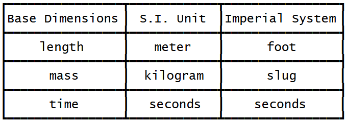
In Physics, the metric system (S.I. units) is the industry standard, and even then, units are converted using conversion factors (see "Dimensional Analysis") into their base dimensions.
#
P. Rule .
When doing a problem, ALWAYS convert all given units into the base S.I. Units unless told otherwise - see the "Units & Dimensions" blue section for these base units. There is a purpose for this beyond what custom has strictly divided - several units are defined in terms of the base units (like Joules in Section VII).
Generally, this will be your first step in any Physics problem involving non-base units, unless the question expressly states that the answer must be given in terms of non-base units. Either way, you need to standardize all dimensions in your problem into the same unit, like having every weight value in kilograms.
Generally, this will be your first step in any Physics problem involving non-base units, unless the question expressly states that the answer must be given in terms of non-base units. Either way, you need to standardize all dimensions in your problem into the same unit, like having every weight value in kilograms.
# Dimensional Analysis:
Being comfortable in performing Dimensional Analysis (conversion from one unit of measurement to another) is critical to all of Physics; it is the underlying prerequisite concept which all problems assume knowledge of.
Dimensional Analysis is conducted using conversion factors, which are just ratios of units that, when multiplied to the original unit, allow you to change the unit without changing the quantity. They allow you to cancel out the original unit, leaving you with the desired one. For example, in converting from hours to seconds,
(2 hours) x (60 min/1 hour) x (60 sec/1 min)
has (60 min/1 hour) and (60 sec/1 min) as the conversion factors, converting from hours to minutes and then minutes to seconds, respectively.
The conversion factor is the fraction being multiplied regardless of the coefficient of the original unit, as shown in how two minutes, 40 minutes, and 542 minutes will all have the same conversion factor when converting into seconds.
Conversion factors, thus, include the desired final unit (or atleast a unit closer to the unit you are trying to get to) in the equivalent ratio with the previous unit, either the one you started with or the previous unit in the conversion factor sequence. Inherently, every conversion factor must equal to one, as the top and bottom are the same value, just expressed in different ways.
#
P. Rule .
When converting one exponentiated unit (², ³, etc.) into another using dimensional analysis, put the exponent on the outside of the parenthesis of the conversion factor (see "Dimensional Analysis" blue section), applying the exponent to the top and bottom in order to allow units to cancel out:
12 mm² → m² = 12 mm² × ((1 m) / (1000 mm))²
= 12 mm² × ((1 m)² / (1000 mm)²)
= 12 mm² × ((1 m²) / (1000000 mm²))
= (1.2 x 10⁻⁵) m²
12 mm² → m² = 12 mm² × ((1 m) / (1000 mm))²
= 12 mm² × ((1 m)² / (1000 mm)²)
= 12 mm² × ((1 m²) / (1000000 mm²))
= (1.2 x 10⁻⁵) m²
# Density:
The density d of a material (the amount of mass in a given space) is the mass per unit volume:
d = (m / V)
Much of the time, an object's density will be described in the base metric units (see the "Units & Dimensions" blue section). As such, densities tend to be given with the units kilograms per cubic meter (kg/m³).
Other metric units will occasionally be used in defining a density: The density of water, for example, is 1.00 gram per cm³. In a problem, unless stated otherwise, these values should be converted into base units to establish uniformity (as stated in Rule 1).
# Dimensional Analysis Comprehension Problem:
Here is an example problem that should not pose too much of an issue to any beginning physicist well-versed in dimensional analysis:
Iron has a density of 7.87 g/cm³, and the mass of an iron atom is 9.27 × 10⁻²⁶ kg. If the atoms are spherical and tightly packed,
(a) what is the volume of an iron atom and
(b) what is the distance between the centers of adjacent atoms?
Answer(s):
a) 1.18 × 10⁻²⁹ m³
b) 2.82 × 10⁻¹⁰ meters
Explanation:
The first step of any Physics problem, as noted in Rule 1, is to convert all measurements into the same units. As the question gives no preference as to what units the answer should be presented, base units should be presumed, and so we will first convert the grams to kilograms and the cubic centimeters to cubic meters:
dI = (7.87 g/cm³) × (1 kg / 1000 g) × (100 cm / 1 hr)³
dI = 7.87 × 10³ kg/m³
Now, the actual problem-solving part of the problem can commence. In order to actually find the volume of the iron atom for part a), one must remember the density equation (described in the "Density" blue section): d = (m / V). Thus, the first and only step for part a) would be to isolate the volume, since the density and mass is already known.
V = (m / dI)
V = (9.27 × 10⁻²⁶ kg) / (7.87 × 10³ kg/m³)
This gives us a result of 1.18 × 10⁻²⁹ m³ for the volume of an iron atom.
Next, for part b), we need to find the distance between the centers of adjacent atoms. Using critical thinking, we can determine that this distance is in fact the diameter of the atom, which we can reverse engineer by isolating the radius from the volume equation of a sphere:
Volume of sphere = (4/3) × π × r³.
r = ∛(3V / 4π)
Plugging in the known volume from answer a), we find that the radius is equal 1.41 × 10⁻¹⁰ meters. Since we are looking for the diameter, we multiply this distance by two and get 2.82 × 10⁻¹⁰ meters.
#
P. Rule .
SIGNIFICANT FIGURES:
'Significant Figures', also known as the Digits of Precision, are the digits within a number that indicate how precise a measurement can be ascertained to be. If a recipe calls for has 1 teaspoon of sugar, you could probably eyeball it, but if it calls for 1.000000 teaspoons of sugar, that's a lot more precise; you'd probably need a laboratory-level scale to get that exact of a measurement.
With significant figures, often abbreviated to sig. fig.'s, perceived preciseness only translates to genunine preciseness half of the time. Below is a simple set of guidelines to follow when determining how many sig. fig.'s are in any number:
#1) All Non-zero digits are significant.
#2) Zeros between significant digits are significant.
#3) Zeros to the left of nonzero digits are not significant.
#4) Zeros at the end of a number are significant only if there is a decimal point present.
The given values, 1 and 1.000000 have different numbers of sig. fig.'s, 1 and 7 respectively, and thus have differing levels of preciseness. However, note that under these immutable guidelines, 0.00001 and 1 have the same number of sig. fig.'s, because zeroes to the left of nonzero digits are not significant (#3).
In Physics, it is convention to use sig. fig.'s in all numerical answers, with the number of significant figures in the answer being equal to the least number of figures in any of the numerical values given in the question. However, never use sig. fig.'s to alter the values used in your actual calculations; only use them to alter your final answer, and even thereafter, if you need to use that answer in another part of the problem, use the un-sigfig'd version to perform your calculations.
Examples:
0.000001 has ONE sig. fig., as a result of guideline 3.
1200 with 3 significant figures: 1.20 x 10³
0.002 with 3 significant figures: 2.00 x 10⁻³
#
P. Rule .
THE ARCANE ROUNDING RULE:
When rounding, if the number ends in a perfect 5, round to the even number.
Examples:
275 with 2 Significant figures: 280
1030 x 5.1 = 5300
When rounding, if the number ends in a perfect 5, round to the even number.
Examples:
275 with 2 Significant figures: 280
1030 x 5.1 = 5300
# Atomic Mass Units:
An additional unit of measurement (derived from kg) specific to atoms (and only occasionally relevant to elementary Physics) is the Atomic Mass Unit, defined as the "atomic mass" of each element in relation to that of Carbon-12. Specifically, Carbon-12 is defined as having 12 amu, and other atoms are calculated in relation to how much mass they have in relation to Carbon-12.
For those familiar with stoichiometry, the amu can be converted to moles easily.
For Mechanics and Electromagnetism, idealized particles or electrons/protons are generally used instead of atoms of a specific element, so for now, only a more peripheral understanding of amu is needed. This relative disregard lasts until higher level Nuclear Physics, which has more of an emphasis on that sort of thing.
# Vertical Scaling:
When you have a problem that makes reference to the vertical or horizontal scaling of a graph (such as the one shown below), the "vertical scaling" is just referring to what the given height value is as each y-value is multiplied by a constant, creating a ratio between the new and original scales.
The old scale will almost always be a scaling of 1:1 (i.e. the normal graph), and the new scale will have a scaling ratio determined by the vertical scaling and its positioning on the graph.
For example, the new scale as depicted in the graph below has a ratio of 2:1 with the old scale, demonstrated by how vs is eight units upward, meaning each unit is two. The exact same process can be applied to the x-axis, resulting in Horizontal Scaling.

#
P. Rule .
Coordinate/Direction Types:
There are three types of directions/coordinates that are critical to one's directional understanding in Physics and life in general: Cartesian, Relative, and Cardinal.
Cartesian Coordinates: (x, y).
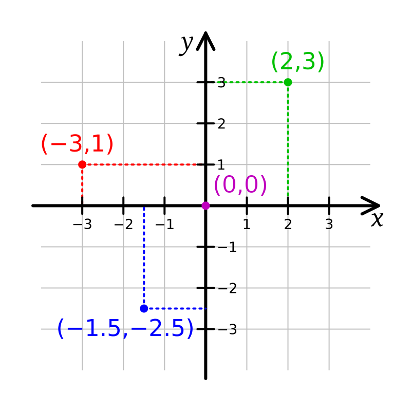 A graph with random cartesian coordinates. Courtesy of GIS.
Relative Coordinates: (Left, Right).
 A graph with relative directions like right and back superimposed over it.
Cardinal Direction: (North, South)
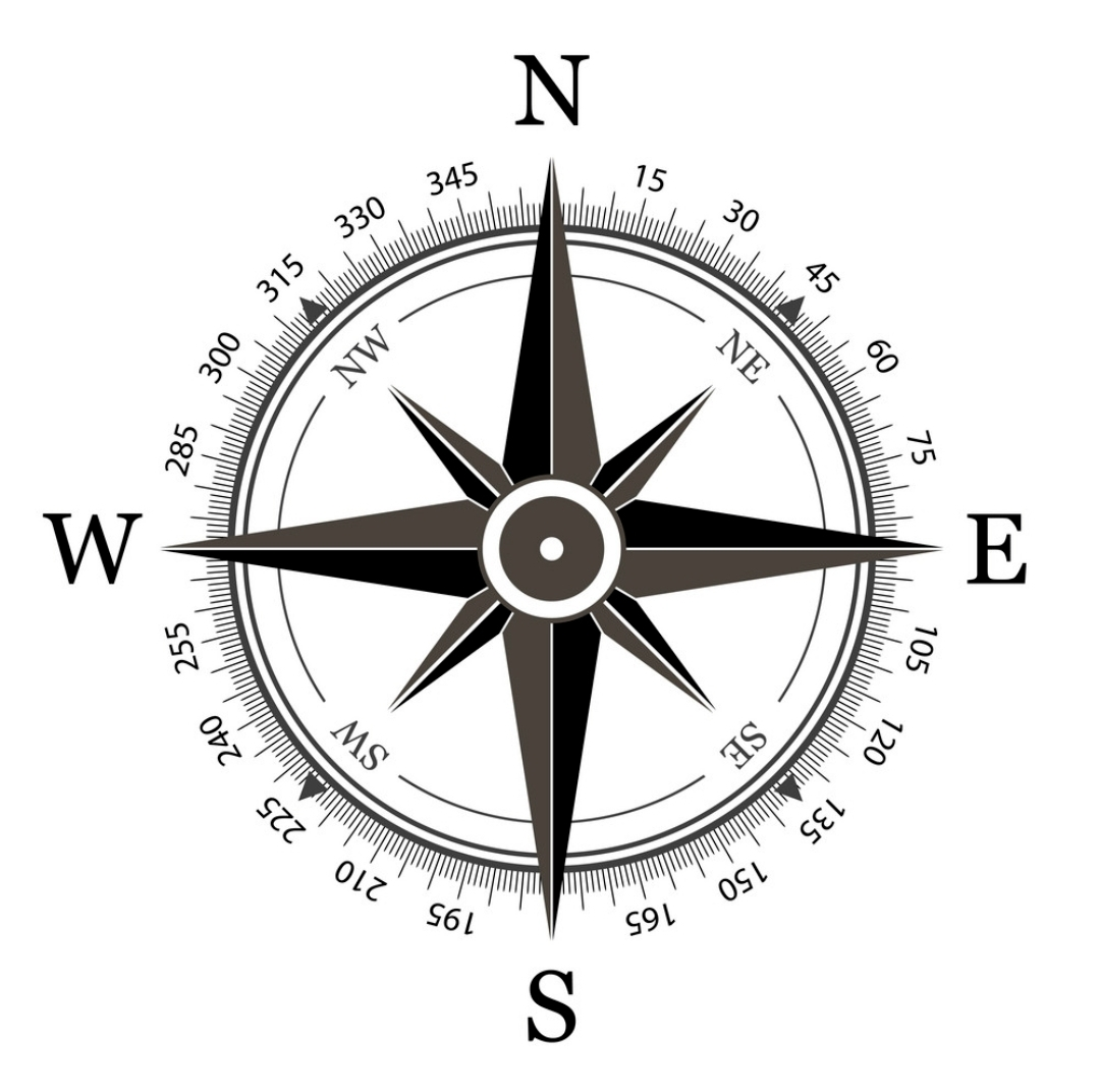 A compass, with each of the cardinal directions labeled.
There are three types of directions/coordinates that are critical to one's directional understanding in Physics and life in general: Cartesian, Relative, and Cardinal.
Cartesian Coordinates: (x, y).
Relative Coordinates: (Left, Right).
Cardinal Direction: (North, South)
I.II Accuracy & Uncertainty.
# Precision: How close the observed/measured values are to one another.
# Relative Error: A measure of accuracy.
Er = ((O - A) / A) × 100
Er = Relative Error. Measures the accuracy of the observed value in relation to the accepted value. Explicitly, it is a percentage representation of the difference between the accepted value and the observed value.
O = Observed Value. If it perfectly matches the accepted value, then there is no error and the Er is equal to 0.
A = Accepted Value.
#
P. Rule .
When finding the accuracy of a selection of observed values, know that you must take an average, either at the beginning or end of your calculations.
For the beginning, you can just take the average of all the observed values immediately, and then use that value as your Observed Value (O) variable in the Relative Error equation (see the "Relative Error" blue section) to find the accuracy.
For the end, you can take the average of all the relative errors, each of which is calculated using one of the observed values. It should give you the same answer as averaging the observed values in the beginning.
Either way, as a result of taking an average of the results, a bullseye that looks like this:
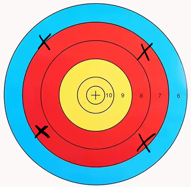 A target with four hits shown medium-distance from the center, forming a high accuracy average.
would be considered to have high accuracy, as they are all equidistant from the middle and thus have their center directly upon it.
For the beginning, you can just take the average of all the observed values immediately, and then use that value as your Observed Value (O) variable in the Relative Error equation (see the "Relative Error" blue section) to find the accuracy.
For the end, you can take the average of all the relative errors, each of which is calculated using one of the observed values. It should give you the same answer as averaging the observed values in the beginning.
Either way, as a result of taking an average of the results, a bullseye that looks like this:
would be considered to have high accuracy, as they are all equidistant from the middle and thus have their center directly upon it.
#
P. Rule .
If there is only one known measured value (that thus cannot be compared to any other measurements), precision cannot be determined.
I.III Uncertainty.
Whenever you are performing a measurement (not a calculation, a MEASUREMENT) in a serious Physics environment, you always need to have an estimated uncertainty to make your work falsifiable.
# Percent Uncertainty: A measure of precision.
Equation:
P = (E / O) × 100
P = The Percent Uncertainty, a measure of precision. The closer the value to 0%, the more precise the observed value is.
E = The Estimated Uncertainty, a.k.a. the number immediately following the ±.
O = The Observed Value.
Definition: The ratio between the estimated uncertainty and the measured value, made into a percentage.
The given equation for percent uncertainty is remarkably similar to the relative error equation, the difference lying in how percent uncertainty only conveys the possible error (uncertainty) in the observed value as a proportion of the observed value itself, while relative error conveys the percentage of the difference between the observed value and the accepted value as a proportion of the accepted value.
Percent uncertainty is a measure of precision through how the answer shows how close the observed and accepted values are to one another (the closer the answer is to 0%, the more precise the observed value is).
For example, with the measurement 8.8 ± 0.1 m, the percent uncertainty would be ((0.1) / (88)) × 100% ≈ 1%.
#
P. Rule .
If a questions asks for the approximate uncertainty (see "Estimated Uncertainty" definition) of something, but gives no hints on how to find it, assume ±1 unit at the lowest digit of precision (under sig. fig. rules given in Rule 3). Additionally, any and all scientific notation on the original value must be extended to all estimated uncertainty assumptions. For example, if the question gives a value of 4.19 × 10³ m, then an estimated uncertainty of 0.01 × 10³ should be presumed.
However: Know that, in practically all cases, this ±1 of whatever unit is not the answer they are looking for. The question will oftentimes phrase the question cleverly, asking for the approximate uncertainty of a shape as a whole but only giving the radius as the given value, causing the ±1 assumption to only be in reference to the radius and requiring additional work to find the approximate uncertainty of the shape.
The question will likely want you to plug in the positive and negative versions of the assumed estimated uncertainty (individually added onto the main value to create two separate values) into another equation in order to find a final approximate uncertainty. This process is detailed in Rule 9, which uses a circle as its example equation.
#
P. Rule .
When you want to find the approximate uncertainty of a 2D shape, use the shape's ideal area formula. If you want to find the approximate uncertainty of a 3D shape, use its volume formula.
For example, if you want to find the approximate uncertainty of a circle given the radius, use πr² as your area formula.
As a general problem example, you are asked to find the approximate uncertainty of a circle with the radius r = 3.8 × 10⁴ m. Of course, A = 4.5 × 10⁹ m². From there, since no percent uncertainty is given, then (as stipulated in Rule 8) you would assume an approximate uncertainty of 0.1 of the original units, ± 0.1 × 10⁴ m. This finds the approximate uncertainty in relation to the radius, but now what must be found is the approximate uncertainty of the circle itself.
From there, you would plug in two values for r into the area equation: the given radius with the approximate uncertainty added (Amax), and with the approximate uncertainty subtracted (Amin). This will produce two distinct areas: Amax = 4.8 × 10⁹. Amin = 4.3 × 10⁹.
At this point, follow this equation: ½(Amax - Amin). Find the difference between the areas, and then divide by 2. This first finds the complete range of the approximate uncertainty of the circle, and then halves it to produce the value that can be placed in front of the ± symbol. This results in a final answer of (4.5 ± 0.24) × 10⁹ m², with ± 0.24 × 10⁹ m² as the circle's approximate uncertainty.
You may wonder whether it would be possible to obtain the final approximate uncertainty by simply finding the difference between Amax and the area using the base radius, circumventing the entire process of finding the difference between both approximate uncertainties and then dividing by two. Sadly, such an idea is too good to be true. This is not feasible as a result of any and all exponential functions in the area/volume equation. If the equation is linear, then it can be done, but it is a better rule of thumb to just always do the process of ½(Amax - Amin) to avoid making unnecesary mistakes.
I.IV Displacement and Velocity, Speed, Acceleration.
# Displacement: The change in position of an object. Mathematically, this means the straight-line distance between the initial and final points, also including direction*. ∆x ("delta-x") is the symbol for displacement and change in position, defined as positionfinal - positioninitial.
Although referred to as ∆x, displacement can have both x and y distance, as ∆x is in reference to position and not just the x-value. This can be somewhat confusing at times, and to add to the confusion, some problems will use ∆x to refer specifically to movement in the x-direction (such as U.A.M. problems, which will be discussed in Subsection I.V), while others use it to refer to positional change as a whole. It is up to you to use your proper judgment to discern the context as to what the ∆x of a problem represents.
*Displacement is a VECTOR (see Section III, on vectors), meaning that it incorporates direction in addition to magnitude. Thus, displacement can be negative or positive, depending on the direction traveled from the initial position. Vectors, as shown below, are depicted with an arrow above the variable.
Unit Vectors are a simplification of x and y positions into their respective directions, detailed in Rule 20. The equation for displacement (using d for displacement) in terms of unit vectors is d = (x₂ - x₁)î + (y₂ - y₁)ĵ
This equation describes displacement in terms of its component vectors on the x-axis and y-axis (see Rule 18). These component vectors indicate the direction and magnitude of the displacement.
In order to find the magnitude of the displacement in the graphical sense, where you have two dots on a graph (the start and end points) and you need to find the straight-line distance between them, you must first find the component vectors in the x and y directions. This will allow you to find the hypotenuse of the right triangle formed by the x and y component vectors (see Rule 18 & Rule 19):
|d| = √((x₂ - x₁)² + (y₂ - y₁)²)
Use this equation when prompted to find the magnitude of the displacement - the direction can be determined by the component vectors themselves; see Rule 20.
#
P. Rule .
NOTE THAT THE DISPLACEMENT EQUATION IS NOT NECESSARY IF THE OBJECT IS ONLY MOVING ALONG A SINGLE AXIS. If the position is only moving along one axis, then you only need to subtract yfinal by yinitial, xfinal by xinitial, or zfinal by zinitial to find displacement.
If not one-dimensional, then the displacement will have to be fully acknowledged as a vector, making use of the given equations above. If the movement is in 2D, then you want to use the magnitude equation as stated, and if it is in 3D, then you should just add + (z₂ - z₁)² is using the magnitude equation or + (z₂ - z₁)k̂ if using the unit vector equation. Useful proof.
If not one-dimensional, then the displacement will have to be fully acknowledged as a vector, making use of the given equations above. If the movement is in 2D, then you want to use the magnitude equation as stated, and if it is in 3D, then you should just add + (z₂ - z₁)² is using the magnitude equation or + (z₂ - z₁)k̂ if using the unit vector equation. Useful proof.
# Total Distance: The cumulative distance traveled between the starting and ending points of the particle.
The total distance traveled will always be greater or equal to the magnitude of displacement, as a result of the fact that total distance accounts for the path taken by the object, and not just the difference between the initial and final positions.
# Velocity: The rate of change of an object's position, utilizing displacement. Velocity has both magnitude and direction (thus making it a vector, described more in Section III), as shown in the below equalities:
Velocity = V
= (∆x / ∆t)
= (xF - xi) / (tF - ti)
= (Change in Position) / (Change in Time)
# Instantaneous Velocity: The velocity at a specific point in time. The Velocityfinal and Velocityinitial from the U.A.M. equations (see section I.V) are instantaneous velocities because they represent the object's velocity at a specific point in time.
# Average Velocity: The velocity over a time period. The velocity definition, change in position over change in time, is an average velocity itself.
#
P. Rule .
An average velocity written as V(5-10 sec) is just (x10 - x5) / (t10 - t5). This style of writing, although can be misinterpreted as meaning V-5 sec, specifies an interval on the graph to find the velocity of.
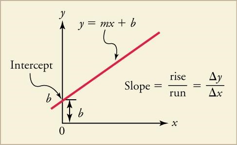
# Slope: The rate of change of a line in a graph, visually identifiable as the steepness of the line. Because the slope is merely a characteristic of a line (its steepness) rather than an actual quantity with direction, it is not a vector and is merely a numerical value (a "scalar", as will described in Subsection III.I).
The steepness of the line at a particular point is the instantaneous slope, better known as the instantaneous velocity (if the line is from the position graph). Below are the equalities for average slope:
Slope = m
= (rise / run)
= (∆y / ∆x)
= (yF - yi) / (xF - xi)
= (Change in Position / Change in Time).
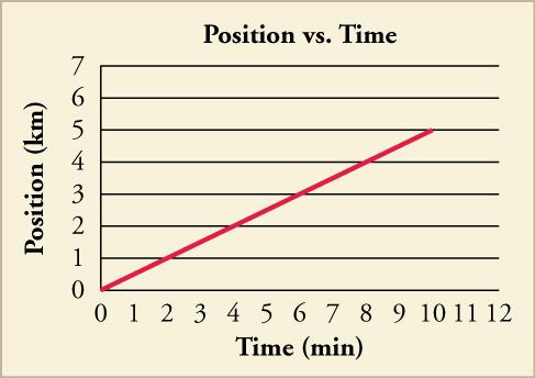
In much the same way as Average Rate of Change (as detailed in the "Average Rate of Change (Contextualized)" blue section), the slope of a "position as a function of the time" graph is the velocity, while the slope of a "velocity vs. time" graph is acceleration. See "The Truth About Velocity & Displacement" for further elaboration.
# Acceleration: The rate of change of velocity. Since velocity is in meters over seconds, acceleration is in in meters per seconds per second, or m/s². Acceleration, as a function of velocity, has both magnitude and direction.
Acceleration = a
= (∆v / ∆t)
= (vF - vi) / (tF - ti)
= (Change in Velocity) / (Change in Time)
Imagine a ball is rolling on an incline, and assume it has a constant acceleration of 2 meters per second squared. What this means is that with each passing second, the velocity will increase by 2 m/s. The ball will start at 0 m/s in velocity and, after 1 second, will get to 2 m/s.
Since this example uses a constant acceleration, finding the position of the ball at each of those times is as simple as using the second U.A.M. equation (detailed in Subsection I.V).
# Average Rate of Change (Contextualized):
When used in different contexts, the 'Average Rate of Change' (A.R.O.C.) can mean different things:
When used in terms of f(x):
A.R.O.C. = Average Velocity = (Displacement / Change in Time).
When used in terms of f'(x):
A.R.O.C. = Average Acceleration = (Change in Velocity / Change in Time).
# Speed: The magnitude-only version of velocity, utilizing the total distance traveled by an object instead of displacement.
Because Velocity accounts for displacement, but speed only for distance traveled, they will only share the same magnitude when the object is moving in a straight line. Velocity specifically uses straight-line distance, so even if the line is curved, the start and end points would still be the only things used to calculate velocity. However, the speed of that curve uses the length of the entire line, all of the distance traveled between point a and point b.
Speed = v
= (total distance) / (time).
As shown above, speed generally uses the same symbol as velocity. The specific symbol being used in a given question is always discernable by the context of the problem.
#
P. Rule .
The object is speeding up whenever velocity and acceleration are in the same direction (e.g. they are the same sign), while it is slowing down whenever velocity and acceleration are in opposite directions/signs.
# The Truth About Velocity & Displacement:
In your reading of Velocity and Slope, you have no doubt encountered these three truths:
Velocity = ∆x / ∆t (Displacement / Change in Time)
Slope = ∆y / ∆x (Change in Y / Change in X)
Velocity = Slope
The '∆x' of the slope equation is not referring to displacement, but rather the change in the x-position. As stated in the displacement definition, ∆x will not uniformly represent displacement in every problem you come across, and even in the given equality there are two different usages of ∆x: displacement and change in x-position. In Physics, you must always use your best judgment to ascertain what the ∆x of a problem represents.
Here are the two equations shown as equivalent:
∆x1 ∆y
━━ = ━━
∆t ∆x2
In addition to knowing that the two equations are equivalent, we know that the ∆x1 of displacement and ∆x2 of slope are not the same, as they refer to displacement and change in x-position, respectively. if we were to cancel out the ∆x of the right side by multiplying it by both sides, we would find that ∆x² / ∆t is equal to ∆y, which is total nonsense.
The key to understanding how the equality is true (and how the ∆x is referring to two things simultaneously) is to realize that both equations are stating the same ratio, just in terms of different graphs.
The equations are both output/input, and they both produce velocity when the slope is calculated between any two points. If the graphs were from the standpoint of velocity, then they would both produce acceleration (see the "Average Rate of Change (Contextualized)" blue section).
I.V Uniformly Accelerated Motion.
Finally, the first unquestionably Physics-specific content can be described after several preliminary sections. All of the previously covered material can be found in other, not necessarily Physics-focused courses, from freshman Calculus to an 8th grade science unit covering the scientific method and uncertainty - now comes the time for the explicit Physics proper, where the skills learned over the previous sections will come into full use.
The following section, regarding Uniformly Accelerated Motion, entails the basic fundamental equations that govern motion (when ignoring things like drag/air resistance - see Subsection III.IV for that), and can be used for both one-dimensional and two-dimensional motion (see Subsection III.III for 2D).
#
P. Rule .
Uniformly Accelerated Motion:
The Uniformly Accelerated Motion (U.A.M.) equations, also known as the Kinematic equations, are a set of four equations that can be used when a given object/system is moving with a constant acceleration. In calculus terms, an object is in constant acceleration when the highest exponent of the position equation is 2 or below (a quadratic or smaller). If the highest exponent is three or above, the object is not in Uniformly Accelerated Motion.
If the position equation is not given, but constant acceleration can be otherwise assumed, U.A.M. can be freely used.
Oft used as a memorization tool for the specifications of U.A.M. is the following mantra: There are 5 U.A.M. variables, and there are 4 equations. If you know 3 variables, you can find the other 2, leaving 1 happy Physics student.
If you are analyzing the movements of two objects, and they share three U.A.M. variable values, then you will know that the other two variables have to be the same as well, and that the movements of the two objects must be identical.
For example, in the classic bullet problem, where a bullet fired horizontally and a bullet dropped from the same height both have a Δy of -h, a y-direction acceleration of -9.81 m/s², and a Viy of 0, it can easily be determined that the rest of the y-direction variables (including the time it would take them to hit the ground) would be the same. This is spite of the fact that the bullets travel different x-distances, as time is the same for the x-direction and y-direction U.A.M. - see Rule 25 and the rest of Projectile Motion for more information.
# U.A.M. Equations:
U.A.M. allows the physicist to use 5 special equations not allowed otherwise. When using the equations, know that they only account for the displacement in a particular direction, and that the variables for movement in the x and y-directions do not necessarily translate between the directions (with the exception of time, as stated in Rule 25).
Solving for any variables (other than time) with regard to movement in one direction does not mean that you can use the values for that variables for the other direction.
For example - if a rocket is launched directly upward, then the Vf of the y-directional movement will be a very large number, while the Vf of the x-directional movement will be 0.
This is very important information, critical for some applications of U.A.M., such as Profectile Motion, which will be covered shortly. In particular, this directional difference is dealt with in more thorough detail in Subsection III.III.
In summary, IN ANY OF THE GIVEN EQUATIONS, YOU CAN CHANGE DISPLACEMENT TO BE CHANGE IN Y IF THE CIRCUMSTANCES OF THE QUESTION DEMANDS IT.
1. VF = Vi + (a × ∆t).
Velocity Final is equal to velocity initial, plus the acceleration multiplied by the change in time.
2. ∆x = (Vi × ∆t) + ½(a × ∆t²)
Displacement is equal to velocity initial multiplied by the change in time, plus 1/2 multiplied by acceleration and the change in time squared.
3. VF² = Vi² + (2 × a × ∆x)
Velocity final squared is equal to velocity initial squared, plus two multiplied by the acceleration and the displacement.
4. ∆x = ½(VF + Vi) × ∆t
The change in position is equal to one half, times the quantity of velocity final plus velocity initial, times the change in time.
VF = Velocity Final (Instantaneous)
Vi = Velocity Initial (Instantaneous)
a = Acceleration
∆t = Change in Time
∆x = Displacement (or change in position)
Additionally, there are some lame 'alternate' versions of these equations using slightly different variables, useful for deriving and integrating the equations:
v = v0 + at
x = x0 + v0t + ½at²
v² = v0² + 2a(x - x0)
x = x0 + ½(v + v0) × t
# Memorization songs for U.A.M. Equations:
<disclaimer>
I believe that the best way to memorize new information is to associate it with something that we have already memorized that we subconsciously reinforce through repetition: music. Everyone has already memorized hundreds of melodies, so finding one that would match the rhythm and meter of the equation is not too terribly difficult. Of course, fast music is most of the time unfit for memorizing an equation, of which a slower recitation and melody are much easier to perfectly and quickly recall.
</disclaimer>
1. To the theme of Funiculì, Funiculà (Slower part):
Vf equals vi + a times change in t.
2. To the theme of Funiculì, Funiculà (Faster Part):
Change in, x equals, vi times change in t. plus one, half times, a, change in t squared.
vi times change in t equals vi times the change in t!
vi times change in t plus one half times a change in t, squared,
vi times change in t plus one half times a change-in-t squared.
3. To the theme of Mozart's Dies Irae:
Vf squared equals, (da da da da) vi squared plus, (da da da da) 2 times a times, change in x equals vi SQUARED plus 2a change in time.
4. To the theme of Satie's Gnossienne No. 5
Delta x, ~~~~ equals one slash two, ~~~~~~~~~~~~~~~ times velocity final plus vi, times change, in time...
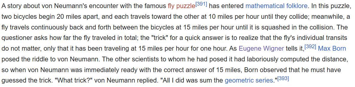
# Esoteric U.A.M. Problem:
A use of the U.A.M. equations that is not immediately apparent:
Two trains, each having a constant speed of 30 km/h, are headed toward eachother on the same straight track. A bird that can fly 60 km/h flies off the front of one train when they are 60 km apart and heads directly for the other train. Upon reaching the other train, the (crazy) bird flies directly back to the first train, and so forth. What is the total distance traveled by the bird before the trains collide?
Answer(s):
60 km
Explanation:
This question has several traits that force the physicist to utilize critical thinking skills instead of just plugging in numbers into formulas mindlessly, which one may get in the habit of if asked too many uninspired questions.
For one, velocity cannot replace speed in most circumstances due to the inherent differences of velocity using straight-line difference and speed using the total distance traveled, but there is one exception: If the object (or objects, in this case) travel in a straight-line, which is to say in one dimension, then the speed is equal to the velocity and they are interchangeable, atleast with regard to magnitude (since velocity is a vector). This is stated in the speed definition.
Utilizing vector addition (see Rule 16) would not work, because the directions would cause the train velocities to cancel out.
The specific parameters of the problem make it easier to solve: imagine the trains as being simple objects with directionless speed (as stated in the problem), for example. From the perspective of the conductor of the first train, the second train is going 60 kilometers per hour, relative to the first train. We can replace the entire two train scenario (which has perfect symmetry and identical U.A.M. variables) and replace it with a single moving object - the trains are individually moving 30 km/hr towards eachother at a starting distance of 60 km from eachother, and as such are equivalent to a single train moving at 60 km/hr toward a brick wall 60 km away. Mathematically, these conclusions can be derived as follows, as a unique result of the symmetry between the movement of the trains:
SpeedTotal = Speed1 + Speed2
SpeedTotal = 30 km/hr + 30 km/hr
SpeedTotal = 60 km/hr
Thus, in this question, ViT and VFT are in reference to the single moving train, and are both equal to 60 km/hr. Additionally, the change in x (displacement) has been changed to 60 km, and considering the doubled speed of the single train, this works out perfectly with the original scenario. Since there are three known U.A.M. variables, we can find the other two.
For this question only, it is more logical to remain in km/hr instead of converting into m/s as is the usual.
We will first try to determine the acceleration using the train's U.A.M. equations - each U.A.M. equation has acceleration, so it is needed to get what is really wanted: the change in time.
VF1² = Vi1² + 2 × a × ∆x
(60 km/hr)² = (60 km/hr)² + 2 × a × 60 km.
0 = 2 × a × 60 km.
a = 0
This simplifies things significantly, and was totally obvious considering that the final velocity is the same as the initial velocity. Thus, for the second equation, which has two parts, both with the change in time (and the second with acceleration as a multiplier, nullifying it), the 2nd U.A.M. equation is best suited for this scenario, as it can quickly isolate the change in time.
∆x = Vi1 × ∆t + ½(a × ∆t²)
60 km = (60 km/hr) × ∆t
∆t = 1
This is the last real mathematical step - lastly, some dreaded logic must be performed. If we were to consider the flying bird, we would find that it is flying at the same speed as the train and would thus go 60 km/hr for one hour before crashing into the wall, which is clearly equal to 1 hours worth of flight and thus 60 km of flight distance. Regardless of the original red herring complexity of how the bird would be moving back and forth between the trains, all one really needs to understand is that the bird will fly for 60 minutes at 60 km/hr before the trains hit eachother. Indeed, this problem has a hidden trick to solving it, although it is not necessary for some.
# WARNING:
KNOWLEDGE REGARDING CALCULUS-CONCEPTS SUCH AS DERIVATIVES WILL BECOME FULLY PREREQUISITE IN THE NEXT PHYSICS SECTION (II). MAKE SURE YOU KNOW ATLEAST THE DERIVATIVE PART OF SINGLE-VARIABLE CALCULUS BEFORE CONTINUING ONTO FREE FALL.

